Categorical Data Analysis for Social Scientists
Table of Contents
- 1. Introduction
- 2. Logistic regression
- 2.1. The linear probability model vs the logistic transformation
- 2.2. Logistic regression: transformation and error
- 2.3. Getting predicted values
- 2.4. Interpretation
- 2.5. Example: Credit card data
- 2.6. Inference: Wald and LRtest in context of multiple variables
- 2.7. Maximum likelihood
- 2.8. Logit for grouped data
- 2.9. Model fit
- 2.9.1. The importance of model fit?
- 2.9.2. Classification tables
- 2.9.3. Classification table for creditcard data
- 2.9.4. Misleading: Even the null model classifies well
- 2.9.5. Sensitivity & specificity
- 2.9.6. Changing cutpoints
- 2.9.7. LROC curve for credit card data
- 2.9.8. Hosmer-Lemeshow statistic
- 2.9.9. Fitstat: Pseudo-R2, BIC
- 2.9.10. Summary: How important is fit
- 2.10. Latent variable approach, probit, cloglog
- 2.11. Issues with logistic regression
- 3. Margins and graphical representations of effects
- 3.1. What are marginal effects?
- 3.2. Non-linear effects
- 3.2.1. Example: quadratic effect in linear regression
- 3.2.2. Marginal effects on a quadratic effect
- 3.2.3. Logistic regression is naturally non-linear
- 3.2.4. Marginal effect in logistic
- 3.2.5. Margins "at means"
- 3.2.6. Average Marginal Effects
- 3.2.7. Big advantages in "truly" non-linear models
- 3.2.8. Age and sex: different marginal effect of age by sex
- 3.2.9. Marginal effects
- 4. Multinomial logistic regression
- 5. Ordinal logit
- 5.1. Stereotype logit
- 5.2. Proportional odds
- 5.2.1. The proportional odds model
- 5.2.2. The model
- 5.2.3. \(J-1\) contrasts again, but different
- 5.2.4. An example
- 5.2.5.
- 5.2.6. Interpretation
- 5.2.7. Linear predictor
- 5.2.8. Predicted log odds
- 5.2.9. Predicted log odds per contrast
- 5.2.10. Predicted probabilities relative to contrasts
- 5.2.11. Predicted probabilities relative to contrasts
- 5.2.12. Inference
- 5.2.13. Testing proportional odds
- 5.2.14. Brant test output
- 5.2.15. What to do?
- 5.2.16. Generalised Ordinal Logit
- 5.3. Sequential logit
- 6. Special topics: depend on interest
1 Introduction
1.1 What this is
1.1.1 About these notes
- These are the notes to go with the short course, "Categorical Data Analysis for Social Scientists", offered on May 14-15 2012, by the Dept of Sociology, University of Limerick
- The course is designed and taught by Dr Brendan Halpin
- The software used is Stata
- The course draws on Regression Models for Categorical Dependent Variables using Stata by J Scott Long and J Freese
- Queries to Brendan Halpin,
brendan.halpin@ul.ie
1.1.2 Online material
- These notes are available at http://teaching.sociology.ul.ie/categorical/
- Lab notes are at http://teaching.sociology.ul.ie/categorical/labs.html and http://teaching.sociology.ul.ie/categorical/labs.pdf
1.2 Association in tables
1.2.1 Social science data is typically categorical
- Much data in the social sciences is categorical – binary, multi-category, ordinal, counts
- The linear regression family is designed for continuous dependent variables: important paradigm but often inappropriate
- We need methods for handling categorical data, especially categorical dependent variables: logistic regression and related techniques
1.2.2 Categorical data needs tables
- But categorical data is primarily data that suits tabular analysis, and thinking in tabular terms runs through categorical data analysis
- Tabular analysis is at once very accessible, simple, easy to communicate \(\ldots\)
- and the basis for much of the more sophisticated techniques
1.2.3 Association in tables
- We see association in tables: the distribution of one variable varies with the values of another
 Highest educational |         sex
       qualification |      male     female |     Total
---------------------+----------------------+----------
           3rd level |     2,890      3,006 |     5,896
Complete second plus |       799      1,048 |     1,847
   Incomplete second |     1,308      1,758 |     3,066
              Low/No |       947      1,448 |     2,395
---------------------+----------------------+----------
               Total |     5,944      7,260 |    13,204
1.2.4 Tables with percentages
- We see it more clearly in percentage patterns
. tab educ rsex, col nofreq

 Highest educational |         sex
       qualification |      male     female |     Total
---------------------+----------------------+----------
           3rd level |     48.62      41.40 |     44.65
Complete second plus |     13.44      14.44 |     13.99
   Incomplete second |     22.01      24.21 |     23.22
              Low/No |     15.93      19.94 |     18.14
---------------------+----------------------+----------
               Total |    100.00     100.00 |    100.00
1.3 Statistical tests for association
1.3.1 Testing for association
- We test for association (\(H_0\): no association) using the \(\chi^2\) test
- Compare observed counts with expectation under independence: \(E_{ij} = \frac{R_i C_j}{T}\)
- Pearson \(\chi^2\) statistic: \(\sum \frac{(O-E)^2}{E}\)
- This has a \(\chi^2\) distribution if the null hypothesis is true, with \(df = (r-1) \times (c-1)\)
- Tests such as Gamma statistic for ordinal association: count concordant and discordant pairs, \(-1 \le \gamma \le +1\), asymptotically normally distributed
1.3.2 Gamma and Chi-2
. tab educ rsex, gamma chi

 Highest educational |         sex
       qualification |      male     female |     Total
---------------------+----------------------+----------
           3rd level |     2,890      3,006 |     5,896
Complete second plus |       799      1,048 |     1,847
   Incomplete second |     1,308      1,758 |     3,066
              Low/No |       947      1,448 |     2,395
---------------------+----------------------+----------
               Total |     5,944      7,260 |    13,204

          Pearson chi2(3) =  76.2962   Pr = 0.000
                    gamma =   0.1182  ASE = 0.014
1.4 Looking at patterns of association
1.4.1 Patterns of association
- Percentages give us the basic information
- Pearson residuals (\(\frac{(O-E)}{\sqrt E}\)) and standardised residuals as improvement over pcts.
- Pearson residuals are the square-root of the cell's contribution to the \(\chi^2\) statistic
- Standardised or adjusted residuals are Pearson residuals scaled to have an approximately standard normal distribution: if the null hypothesis is true most will fall with the range \(\pm 2\) and any outside \(\pm 3\) are worth noting
1.4.2 Observed and expected
. tabchi educ rsex
-----------------------------------------
Highest educational  |        sex
qualification        |     male    female
---------------------+-------------------
           3rd level |     2890      3006
                     | 2654.182  3241.818
                     |
Complete second plus |      799      1048
                     |  831.458  1015.542
                     |
   Incomplete second |     1308      1758
                     | 1380.211  1685.789
                     |
              Low/No |      947      1448
                     | 1078.149  1316.851
-----------------------------------------
1.4.3 Standardised residuals are approximately normal
. tabchi educ rsex, adj noo noe

          adjusted residual

-------------------------------------
Highest educational  |      sex
qualification        |   male  female
---------------------+---------------
           3rd level |  8.298  -8.298
Complete second plus | -1.637   1.637
   Incomplete second | -2.992   2.992
              Low/No | -5.953   5.953
-------------------------------------

          Pearson chi2(3) =  76.2962   Pr = 0.000
 likelihood-ratio chi2(3) =  76.4401   Pr = 0.000
1.5 Measures of association
1.5.1 Measures of association
In the 2x2 case, we can focus on simple measures of association:
- difference in percentages
- ratio of percentages ("relative rate")
- Odds ratio
Difference in percentages are intuitive: men's achievement of 3rd level qualification is 48.6\% versus women's 41.4\%: a difference of 7.2\%
However, it is more reasonable to think in multiplicative terms: 48.6/41.4 = 1.17, implying men are 17\% more likely to achieve 3rd level.
But the ratio of odds has better properties than the ratio of rates
1.5.2 Odds ratios
Odds: proportion with divided by proportion without
- Men: 2890 / (5944 - 2890) = 0.946
- Women: 3006 /(7260 - 3006) = 0.707
- Odds ratio: 0.946 / 0.707 = 1.339
Men's odds are 1.339 times as big as women's.
The odds ratio is symmetric, and is thus more consistent across the range of baseline probabilities than the relative rate.
The relative rate is easy to communicate: "men are X times more likely to have this outcome than women"; but it does not relate well to the underlying mechanism
1.5.3 RRs and ORs
- Consider a relative rate of 2.0: men twice as likely
| Women's rate | Men's rate |
| 1% | 2% |
| 10% | 20% |
| 40% | 80% |
| 55% | 110% |
- There is a ceiling effect: the relative rate is capped.
- If the OR is 2:
| Women's rate | Women's odds | Men's odds | Men's rate |
| 1% | 1/99 | 2/99 | 1.98% |
| 10% | 1/9 | 2/9 | 18.2% |
| 40% | 2/3 | 4/3 | 57.1% |
| 55% | 11/9 | 22/9 | 70.1% |
| 90% | 9/1 | 18/1 | 94.7% |
1.5.4 ORs and larger tables
- ORs are concerned with pairs of pairs categories, 2x2 tables
- Once we know the margins (row and column totals) of a 2x2 table there is only one degree of freedom: we can complete the table knowing one additional piece of information
- This could be a cell value, or a measure of association such as a difference in proportion, a relative rate or an odds ratio
- A larger table has \( (r-1) \times (c-1) \) degrees of freedom, and can be described by that number of ORs or other pieces of data
- That is, the structure of association in table can be described by \( (r-1) \times (c-1) \) ORs
- ORs are mathematically tractable, and are used in several useful models for categorical data
2 Logistic regression
2.1 The linear probability model vs the logistic transformation
2.1.1 Predicting probability with a regression model
If we have individual level data with multiple variables that affect a binary outcome, how can we model it?
The regression framework is attractive:
\[ Y = f(X_1, X_2, \ldots , X_k) \]
The Linear Probability Model is a first stop: \[ P(Y=1) = \beta_0 + \beta_1 X_1 + \beta_2 X_2 \ldots + \beta_k X_k \sim \mathcal{N}(0,\sigma^2) \]
- Considering the \(\hat Y\) as a probability solves the continuous–binary problem
- But errors are not normally distributed
- And predictions outside the [0,1] range are possible
2.1.2 LPM: residuals and predictions
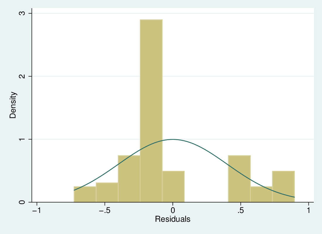
Predicting the probability of possessing a credit card, given income, (Agresti \& Finlay, Ch 15).
2.1.3 LPM output
. reg card income

      Source |       SS       df       MS              Number of obs =     100
-------------+------------------------------           F(  1,    98) =   34.38
       Model |  5.55556122     1  5.55556122           Prob > F      =  0.0000
    Residual |  15.8344388    98  .161575906           R-squared     =  0.2597
-------------+------------------------------           Adj R-squared =  0.2522
       Total |       21.39    99  .216060606           Root MSE      =  .40197

------------------------------------------------------------------------------
        card |      Coef.   Std. Err.      t    P>|t|     [95% Conf. Interval]
-------------+----------------------------------------------------------------
      income |   .0188458    .003214     5.86   0.000     .0124678    .0252238
       _cons |  -.1594495    .089584    -1.78   0.078    -.3372261     .018327
------------------------------------------------------------------------------
2.1.4 LPM not ideal
- The LPM therefore has problems
- Can be worse with multiple explanatory variables
- However, when predicted probabilities are not extreme (say 0.2 – 0.8), it can be effective, robust and easy to communicate
- Note the LPM is working with an additive model, difference in rate rather than relative rate or odds ratio: a 1-unit increase in X adds \(\beta\) to the predicted probability
2.2 Logistic regression: transformation and error
2.2.1 The logistic regression model
- The logistic regression model avoids these problems with two elements
- a transformation of the relationship between the dependent variable and the linear prediction, and
- a binomial distribution of the predicted probability
- The logistic transformation maps between the [0,1] range of
probability and the \((-\infty, \infty)\) range of the linear predictor
(i.e., \(\alpha + \beta x\)):
- odds = \(\frac{p}{1-p}\) maps [0,1] onto \([0, \infty)\)
- log-odds maps \([0, \infty)\) onto \((-\infty, \infty)\)
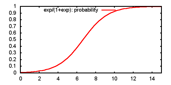
2.2.2 The "Sigmoid Curve"
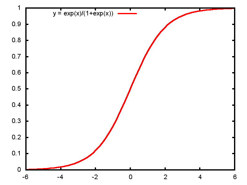
2.2.3 The logistic regression model
\[ \log \frac{P(Y=1)}{1-P(Y=1)} = \alpha + \beta x \] or \[ P(Y=1) = \mathsf{invlogit}(\alpha + \beta x) \sim \mathsf{binomial} \]
2.3 Getting predicted values
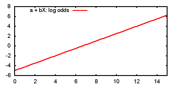
2.3.1 Predicted log-odds
\[ \log \frac{P(Y=1)}{1-P(Y=1)} = \alpha + \beta x \]
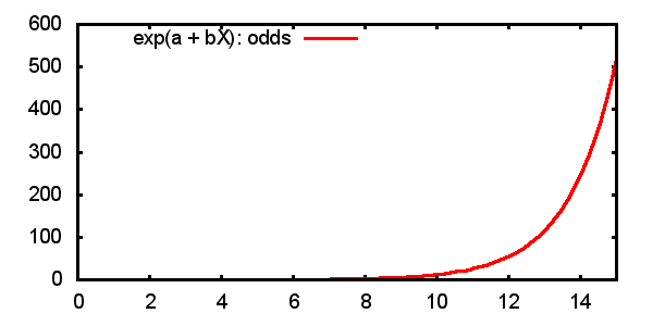
2.3.2 Predicted odds
\[ \frac{P(Y=1)}{1-P(Y=1)} = \mathsf{odds}(Y=1) = e^{\alpha + \beta x} \]
2.3.3 Predicted probabilities
\[ P(Y=1)= \frac{e^{\alpha + \beta x}}{1+e^{\alpha + \beta x}} = \frac{1}{1+e^{-(\alpha + \beta x)}} \]
2.4 Interpretation
2.4.1 Interpretation of \(\beta\)
In linear regression, a 1-unit change in X leads to a \(\beta\) change in \(\hat Y\).
In logistic regression, a 1-unit change in X leads to
- a \(\beta\) change in the predicted log-odds
- a multiplicative change of \(e^\beta\) in the odds
- a non-linear change in the predicted probability
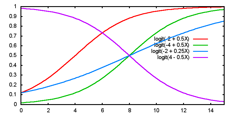
2.4.2 Effects of parameter estimates on predicted probability
2.5 Example: Credit card data
2.5.1 Logit model of credit card data
. logit card income

Iteration 0:   log likelihood = -61.910066
Iteration 1:   log likelihood = -48.707265
Iteration 2:   log likelihood = -48.613215
Iteration 3:   log likelihood =  -48.61304
Iteration 4:   log likelihood =  -48.61304

Logistic regression                               Number of obs   =        100
                                                  LR chi2(1)      =      26.59
                                                  Prob > chi2     =     0.0000
Log likelihood =  -48.61304                       Pseudo R2       =     0.2148

------------------------------------------------------------------------------
        card |      Coef.   Std. Err.      z    P>|z|     [95% Conf. Interval]
-------------+----------------------------------------------------------------
      income |   .1054089   .0261574     4.03   0.000     .0541413    .1566765
       _cons |  -3.517947   .7103358    -4.95   0.000    -4.910179   -2.125714
------------------------------------------------------------------------------
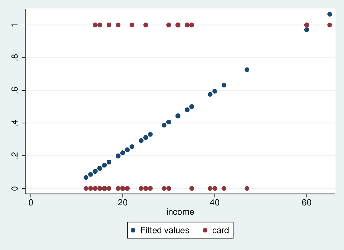
2.5.2 Logistic and LPM predictions
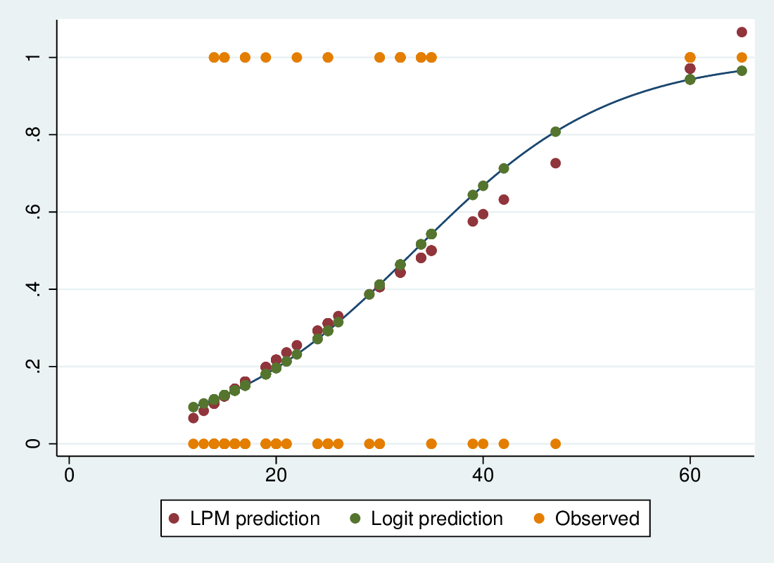
2.5.3 Predictions are similar
- The predictions are quite similar, but logit predictions are all in-range
- The LPM predictions around 40 are probably depressed by the need to keep the predictions around 60 from going even higher
- The LPM says p rises by 0.0188 for a 1-unit rise in income
- The logistic model says the log-odds rise by 0.105 for a 1-unit rise
- This means the odds change by a multiplicative factor of \(e^{0.105} = 1.111\), an increase of 11.1\%
2.6 Inference: Wald and LRtest in context of multiple variables
2.6.1 Inference: \(H_0: \beta = 0\)
- In practice, inference is similar to OLS though based on a different logic
- For each explanatory variable, \(H_0: \beta = 0\) is the interesting null
- \(z = \frac{\hat\beta}{SE}\) is approximately normally distributed (large sample property)
- More usually, the Wald test is used: \(\left(\frac{\hat\beta}{SE}\right)^2\) has a \(\chi^2\) distribution with one degree of freedom – different maths, same numbers!
2.6.2 Inference: Likelihood ratio tests
- The ``likelihood ratio'' test is thought more robust than the Wald test for smaller samples
- Where \(l_0\) is the likelihood of the model without \(X_j\), and \(l_1\) that with it, the quantity \[ -2 \left( \log \frac{l_0 }{l_1} \right) = -2 \left( \log {l_0 } - \log l_1 \right) \] is \(\chi^2\) distributed with one degree of freedom
2.6.3 Nested models
- More generally, \(-2 \left( \log \frac{l_o }{l_1} \right)\) tests nested models: where model 1 contains all the variables in model 0, plus \(m\) extra ones, it tests the null that all the extra \(\beta\)s are zero (\(\chi^2\) with \(m\) df)
- If we compare a model against the null model (no explanatory variables, it tests \[ H_0: \beta_1 = \beta_2 = \ldots = \beta_k = 0 \]
- Strong analogy with \(F\)-test in OLS
2.7 Maximum likelihood
2.7.1 Maximum likelihood estimation
- Unlike OLS, logistic regression (and many, many other models) are extimated by \emph{maximum likelihood estimation}
- In general this works by choosing values for the parameter estimates which maximise the probability (likelihood) of observing the actual data
- OLS can be ML estimated, and yields exactly the same results
2.7.2 Iterative search
- Sometimes the values can be chosen analytically
- A likelihood function is written, defining the probability of observing the actual data given parameter estimates
- Differential calculus derives the values of the parameters that maximise the likelihood, for a given data set
- Often, such ``closed form solutions'' are not possible, and the values for the parameters are chosen by a systematic computerised search (multiple iterations)
- Extremely flexible, allows estimation of a vast range of complex models within a single framework
2.7.3 Likelihood as a quantity
- Either way, a given model yields a specific maximum likelihood for a give data set
- This is a probability, henced bounded [\(0:1\)]
- Reported as log-likelihood, hence bounded (\(-\infty:0\)]
- Thus is usually a large negative number
- Where an iterative solution is used, likelihood at each stage is usually reported – normally getting nearer 0 at each step
2.8 Logit for grouped data
2.8.1 Logistic regression when data is grouped
- If all explanatory variables are categorical, the data set can be reduced to a multi-way table
- If the number of cells in the table is small relative to N, think in terms of blocks of trials
- This won't work with individually variable data
- If the data is naturally grouped, this is also good
- e.g., multiple sites of observation
- m success out on n trials at each site
- site-level covariates
- Examples: Data on number of A-grades and class size for a sample of modules; number of caesarian and total births by hospital
2.8.2 Binomial distribution with a denominator
- In this case, you can consider the outcome as binomially distributed within each setting, as m successes out of n trials
- With individual-data: 0 or 1 success out of 1 trial
- Each setting is treated as a single observation, giving one DF
- "Setting" may be a site of observation, or a unique combination of values of explanatory variables
2.8.3 Model fit with grouped data
- If there are many more cases than settings, we can compare predicted and observed numbers of successes, analogously to Pearson \(\chi^2\)
- Fit a "saturated" model, with as many predictors as settings: predicts the data perfectly
- A LR-test between the working model and the saturated model tests the fit
- The LR-\(\chi^2\) that
tabchireports can be calculated like this - A significant LR \(\chi^2\) test rejects the hypotheses that all the extra parameters in the saturated model have a true value of zero
- That is, your model doesn't fit the data
- An insignificant LR \(\chi^2\) means that your model is consistent with the data
2.9 Model fit
2.9.1 The importance of model fit?
"There is no convincing evidence that selecting a model that maximises the value of a given measure of fit results in a model that is optimal in any sense other than the model's having a larger value of that measure."
Long & Freese, p154
- Nonetheless, there are a lot of ways people try to assess how well their model works
- Straightforward with grouped data
- Other approaches:
- Classification tables
- Sensitivity, specificity and ROC analysis
- Pseudo-\(R^2\)
- Hosmer-Lemeshow statistic
2.9.2 Classification tables
- An obvious way to test model adequacy is to compare predicted and observed outcomes at the individual level
estat classafter a logistic regression gives the table- Predicted \(p>0.5\) is a predicted yes
- Key summary is percent correctly classified
2.9.3 Classification table for creditcard data
. estat class

Logistic model for card

              -------- True --------
Classified |         D            ~D  |      Total
-----------+--------------------------+-----------
     +     |        13             6  |         19
     -     |        18            63  |         81
-----------+--------------------------+-----------
   Total   |        31            69  |        100

Classified + if predicted Pr(D) >= .5
True D defined as card != 0
--------------------------------------------------
[...]
--------------------------------------------------
Correctly classified                        76.00%
--------------------------------------------------
2.9.4 Misleading: Even the null model classifies well
. estat class

Logistic model for card

              -------- True --------
Classified |         D            ~D  |      Total
-----------+--------------------------+-----------
     +     |         0             0  |          0
     -     |        31            69  |        100
-----------+--------------------------+-----------
   Total   |        31            69  |        100

Classified + if predicted Pr(D) >= .5
True D defined as card != 0
--------------------------------------------------
[...]
--------------------------------------------------
Correctly classified                        69.00%
--------------------------------------------------
2.9.5 Sensitivity & specificity
- Sensitivity & specificity are two useful ideas based on the classification
- Sensitivity: P(predict yes | true yes) – a sensitive test has a high chance of correctly predicting a yes
- Specificity: P(predict no | true no) – a specific test has a low chance of incorrectly predicting yes
- A good model or test should have high values on both
2.9.6 Changing cutpoints
- Dividing predictions relative to p=0.5 is intuitively appealing
- But no reason not to use other cutpoints
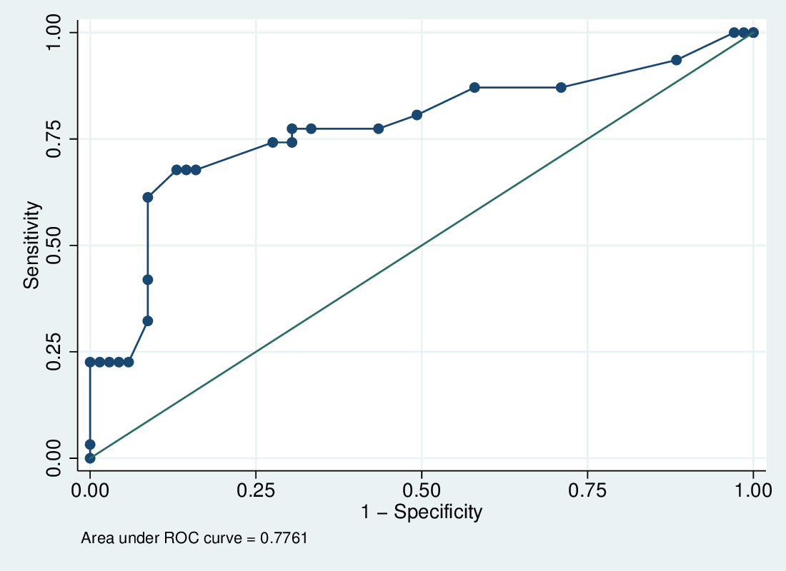
- ROC analysis compares S&S for every value of \(\hat p\) in the data set
- At p=0, 100% yes, so sensitivity is 1 and specificity is 0
- At p=1, 100% no, so sensitivity is 0 and specificity is 1
lrocafterlogitplots sensitivity (true positive rate) against 1-specificity (false positive rate): a trade off- The more the curve tends north-west the better
2.9.7 LROC curve for credit card data
2.9.8 Hosmer-Lemeshow statistic
- With grouped data we can compare predicted and observed values in a tabular manner
- Not with individual data
- The Hosmer-Lemeshow statistic attempts to get an analogous result:
- divide predicted probability into groups (e.g., deciles)
- compare average predicted p and proportion of outcomes within the groups
- A summary statistic based on this is thought to have a \(\chi^2\) distribution with df 2 less than the number of groups
- Results depend on the number of groups
- Useful but not conclusive
- Fuller details, Long & Freese p 155-6
2.9.9 Fitstat: Pseudo-R2, BIC
- Long & Freese's add-on contains the useful
fitstatcommand - Reports many fit statistics after estimating the logistic regression
- Includes a number of "pseudo-\(R^2\)" statistics: ways of faking \(R^2\) based on the log-likelihood – see http://www.ats.ucla.edu/stat/mult_pkg/faq/general/psuedo_rsquareds.htm for a useful overview
- Also reports three versions of BIC – all differ from model to model in exactly the same way, so they're equivalent
- Based on LL, N-cases and n-predictors: penalise model comparison based on LL according to number of predictors; reward parsimonious models
- The model with the lower BIC is "preferred"
2.9.10 Summary: How important is fit
- Don't ignore model fit, but don't sweat it
- It's a hint that you might have missed an important variable, or that another functional form might be good
- The LR-test for model search is good, with clear inference for nested models
- Fit for grouped data has a nice clean interpretation: LR test against the saturated model
- BIC is good for comparing non-nested models as well as nested, rewarding parsimony
- See graphic on p157 L&F: a nice way of looking at fit at the data-point level
2.10 Latent variable approach, probit, cloglog
2.10.1 A latent propensity model
- Assume a latent (unobserved) propensity, \(y^*\), to have the outcome
- Assume it is scaled to have a known variance, and the following relationship to the observed binary outcome
- If explanatory variables have a straightforward effect on \(y^*\):
\[ y^* = \alpha^l + \beta^l X + e \]
- then the logistic model will identify the same relationship:
\[ \log \frac{P(Y=1)}{1-P(Y=1)} = \alpha + \beta X \]
- The relationship between \(\beta\) and \(\beta^l\) depends on the variance
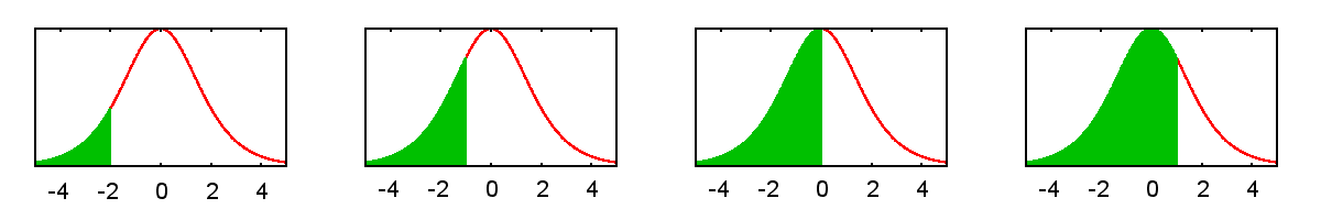
2.10.2 Latent variable and binary outcome
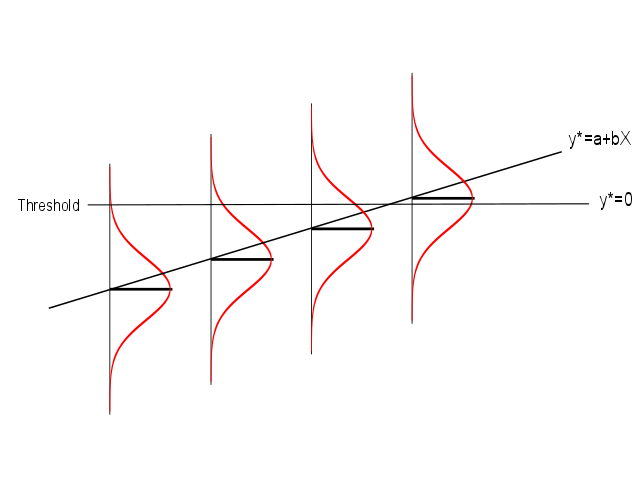
2.10.3 Going up in steps of \(\beta^l\)
- Each 1-unit increase in X increases \(y^*\) by \(\beta^l\)
- Move up the error distribution accordingly
- If the error is logistic (mathematically tractable), P(Y=1) for a given X is \(\frac{1}{1+e^{-(\alpha^l+\beta^lX-\mu)/z}}\) where \(\mu\) is mean and \(z\) is a scale factor
- \(\mu\) is naturally zero; if we set \(z=1\) we get \(\frac{1}{1+e^{-(\alpha^l+\beta^lX)}}\)
- This give \(\beta = \beta^l\)
2.10.4 Logistic and normal distributions
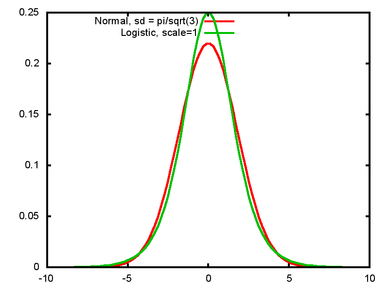
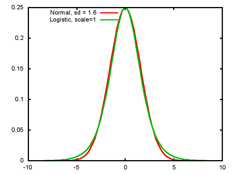
- Logistic distribution with scale 1 has standard deviation = \(\frac{\pi}{\sqrt 3}\)
- Very similar in shape to normal distribution, but mathematically easier to work with
2.10.5 Normal and Logistic CDF
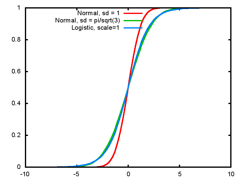
2.10.6 CDF and Probit
- We thus see how we can arrive at the logistic sigmoid curve as a CDF as well as a consequence of the logistic transformation
- With other CDFs, we can have other models
- Probit regression uses the standard normal as the error distribution for the latent variable
\[ P(Y=1) = \Phi(\alpha + \beta X) \]
- Very similar to logistic
- Disadvantage: doesn't have the odds-ratio interpretation
- Advantage: latent variable has a normal distribution
- Parameter estimates smaller, usually by a factor of 1.6 to 1.8 as a consequence of the different scale
2.10.7 Extreme value distribution and cloglog
- Where an outcome is a consequence of prolonged exposure, rather than a 1-off, the distribution is not likely to be logistic or normal
- The chance of having ever married, ever contracted HIV, ever had a flood
- Extreme value distribution is appropriate here (asymmetric)
- A latent variable with an EVD gives rise to the complementary log-log transformation:
\[ \log (- \log(1 - P(Y=1))) = \alpha + \beta X \]
- The \(\beta\) can be interpreted as the effect of X on the log of hazard of the outcome, that is the probability of the outcome, conditional on still being at risk
- When this model is appropriate, logit and probit give biased estimates
2.11 Issues with logistic regression
2.11.1 Issues with logistic regression
Logistic regression is very similar to linear regression in its interpretation but there are special issues
- Separation and sparseness
- Assumption of homoscedasticity of latent variable
- The effect of finite variance on paramater estimates across models
- How to interpret interactions
2.11.2 Separation and sparseness
- Separation: predictor predicts perfectly
- Sparseness: few or no cases in certain combinations of values
- Effectively in certain situations the OR is 0 or \(\infty\)
- Computers can't estimate log-ORs of \(-\infty\) or \(\infty\)
- if left to their own devices will give a large \(\hat\beta\) and an enormous SE
- Stata's
logitcommand is clever enough to identify these situations and will drop cases and variables – very important to see that it does this
. logit own i.educ c.age i.nchild if inrange(age,30,40)

note: 7.nchild != 0 predicts success perfectly
      7.nchild dropped and 2 obs not used
- Sometimes the effect is trivial but sometimes it necessarily drops a very strong predictor
2.11.3 Heteroscedasticity of latent variable
- The latent variable approach depends on the assumption of homoscedasticity
- That is, the error distribution is the same for all values of X
- Affects logit and probit equally
- Stata has
hetprobwhich allows you to add terms to take account of this; see Stata's documentation
2.11.4 Finite variance
- The latent variable approach also works by imposing a fixed variance, \(\frac{\pi^2}{3}\) for logit, 1 for probit
- The size of parameter estimates depends on what else is in the model, in a way that is not true for linear regression
- Adding variables to the model may tend to increase the size of others' effects, even where not correlated
- see Mood (2010) "Logistic Regression: Why We Cannot Do What We Think We Can Do, and What We Can Do About It", European Sociological Review 26(1)
2.11.5 Interactions
- Ai and Norton claim you can't interpret interaction terms in logit and probit:
The magnitude of the interaction effect in nonlinear models does not equal the marginal effect of the interaction term, can be of opposite sign, and its statistical significance is not calculated by standard software. We present the correct way to estimate the magnitude and standard errors of the interaction effect in nonlinear models.
(2003) "Interaction terms in logit and probit models", Economics Letters 80
- Gets echoed as "can't interpret interaction effects in logistic"
- Depends on defining "effect" as "marginal additive effect on predicted probability", & on considering odds-ratios as too obscure & difficult to interpret
2.11.6 Yes, but
- Clearly right in that the effect on \(p\) is non-linear so interaction effects have a complex non-linear pattern
- However, it is perfectly possible to interpret interaction effects as additive effects on the log-odds or multiplicative effects on the odds (effects on the odds ratio)
- Focusing on additive effects on the probability dimension loses a lot of the advantages of the logistic approach
- See also M.L. Buis (2010) "Stata tip 87: Interpretation of interactions in non-linear models", The Stata Journal, 10(2), pp. 305-308. http://www.maartenbuis.nl/publications/interactions.html
3 Margins and graphical representations of effects
3.1 What are marginal effects?
3.1.1 What are marginal effects?
- Under linear regression, a 1-unit change in X leads to a \(\beta\) change in \(\hat Y\): the "marginal effect" is \(\beta\)
- With non-linear models this is not so straightforward
- Calculating "marginal effects" is a way of getting back to a simple summary
3.1.2 Why are marginal effects interesting?
- Representing non-linear effects of vars
- Reducing disparate models to comparable scale
- Communicating, giving a measure of substantive significance
- Warning: don't over-interpret, they're secondary to the main model
3.2 Non-linear effects
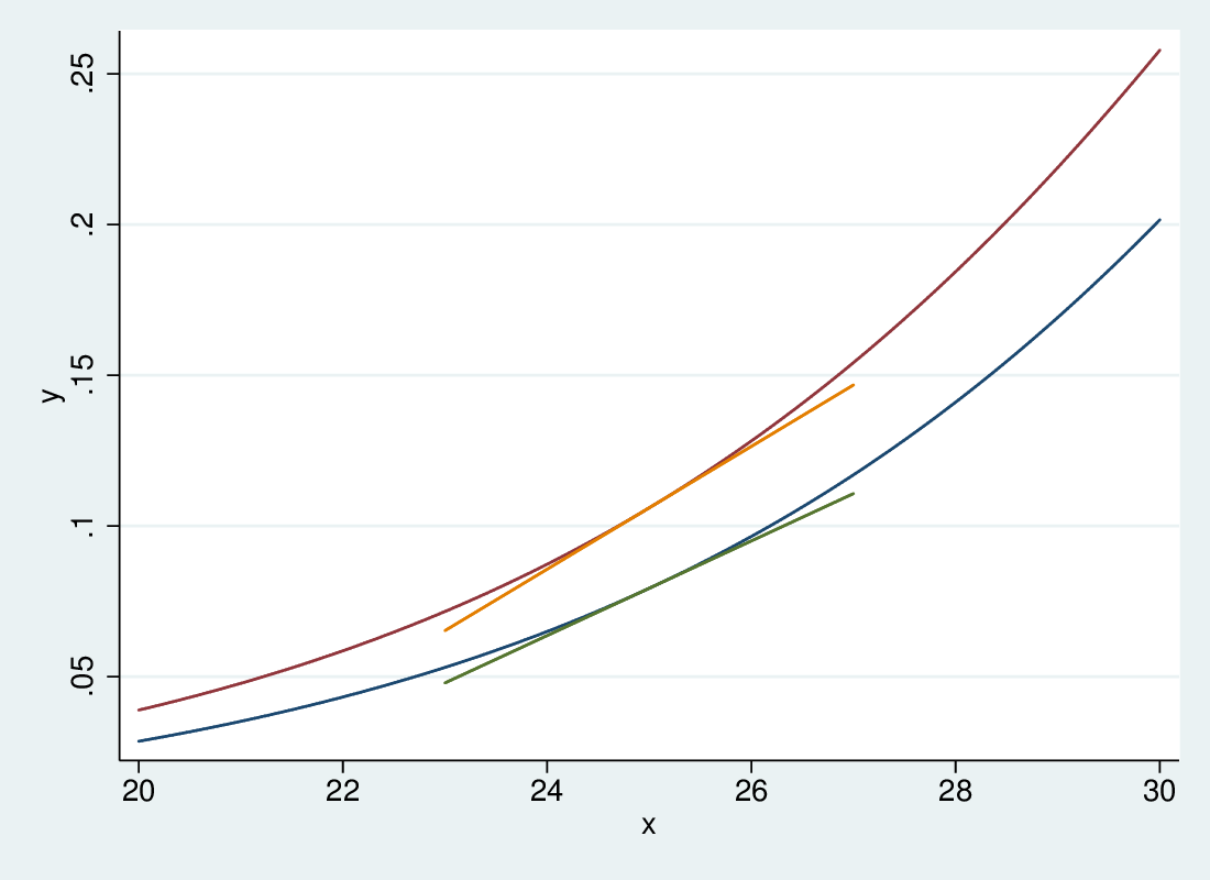
3.2.1 Example: quadratic effect in linear regression
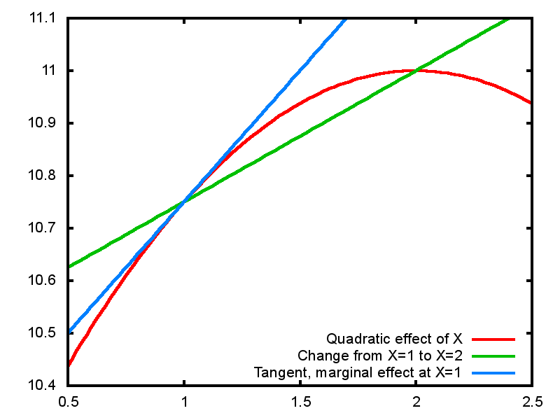
- If we have a squared term in a linear regression that variable no longer has a linear effect: \(Y = a + \beta_1 X + \beta_2 X^2\)
- A 1-unit change in X leads to a change in Y of \(\beta_1 + 2\beta_2 X +\beta_2\) – now the change depends on X!
- We can define the marginal effect as the change in Y for an infinitesimal change in X: this is the differential of the regression function with respect to X, or the slope of the tangent to the curve: \(\beta_1 + 2\beta_2 X\)
- Note that while this depends on X it does not depend on other variables in linear regression (unless there are interaction effects)
3.2.2 Marginal effects on a quadratic effect
\(Y = 10 + 0.5X - 0.25X^2\)
3.2.3 Logistic regression is naturally non-linear
\(\mathsf{logit}(P(Y=1)) = -5 + 0.5X\)
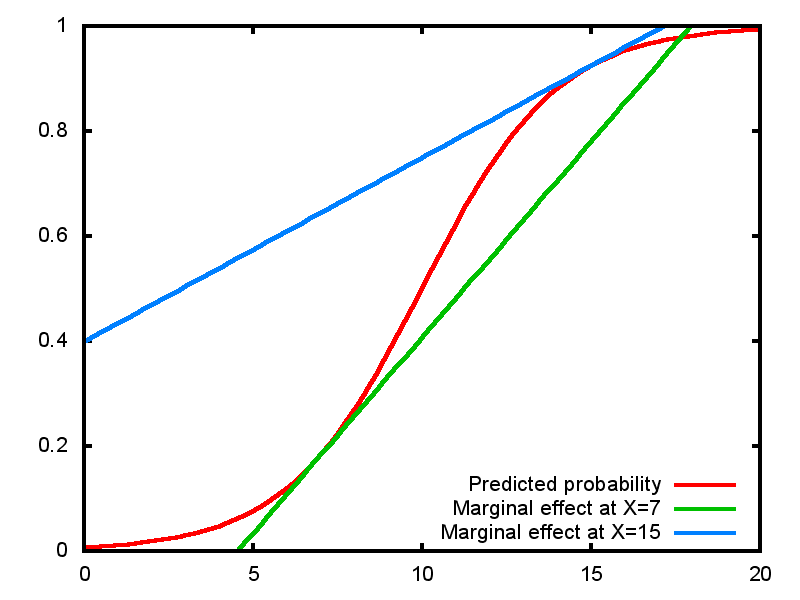
3.2.4 Marginal effect in logistic
- The slope of the tangent is \(\beta p(1-p)\)
- Maximum at \(p=0.5\) at \(\frac{\beta}{4}\)
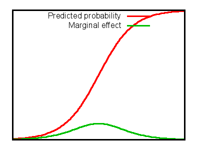
- Depends on X because \(p\) depends on X
- But also depends on all other variables since they also affect \(p\)
3.2.5 Margins "at means"
- In simple regression the effect of a variable has one parameter, \(\beta\)
- With non-linear RHS variables or a non-linear functional form, the effect of a variable is a function in its own right, and can depend on the values of other variables
- Best represented graphically
- But we often want a single summary
- A typical approach: set all other variables to their means (important in logistic, not so much with linear regression), calculate the marginal effect of X at its mean
- May be atypical: could be no cases are near the mean on all variables
- May elide differences, may suggest no effect where there is a strong changing effect
margins, dydx(X) atmeans
3.2.6 Average Marginal Effects
- Second approach is to calculate marginal effect for each observation, using observed values of all variables
- Then average the observation-specific effects for "Average Marginal Effect" (AME)
margins, dydx(X)
- Also, in this case a real effect can appear to be near zero: e.g., where the positive effect at younger ages is offset by the negative effect at older ages
3.2.7 Big advantages in "truly" non-linear models
AME has a bigger pay-off in truly non-linear models where the marginal effect is affected by all variables
- Logistic regression marginal effect is \(\beta*p*(1-p)\)
- Since \(X_1\) affects \(p\), the marginal effect of \(X_1\) varies with \(X_1\)
- But if \(X_2\) is in the model, it also affects the marginal effect of \(X_1\)
- For instance, in a model where sex and age affect the outcome, the marginal effect of age at any given age will differ by sex
3.2.8 Age and sex: different marginal effect of age by sex
3.2.9 Marginal effects
- Average marginal effects can be a useful single-number summary
- Can throw different light from \(\beta\)
- However, they can obscure as much as they enlighten
- Use graphical representation to get a better understanding
- Remember that they are summary of a model, and do not get you away from the underlying structure
- For logistic regression, thinking in terms of effects on odds will get you further than effects on probabilities.
4 Multinomial logistic regression
4.1 baseline category extension of binary
4.1.1 What if we have multiple possible outcomes, not just two?
- Logistic regression is binary: yes/no
- Many interesting dependent variables have multiple categories
- voting intention by party
- first destination after second-level education
- housing tenure type
- We can use binary logistic by
- recoding into two categories
- dropping all but two categories
- But that would lose information
4.1.2 Multinomial logistic regression
- Another idea:
- Pick one of the \(J\) categories as baseline
- For each of \(J-1\) other categories, fit binary models contrasting that category with baseline
- Multinomial logistic effectively does that, fitting \(J-1\) models simultaneously
\[ \log \frac{P(Y=j)}{P(Y=J)} = \alpha_j + \beta_jX, \,\,\, j=1,\ldots,c-1 \]
- Which category is baseline is not critically important, but better for interpretation if it is reasonably large and coherent (i.e. "Other" is a poor choice)
4.1.3 Predicting p from formula
\[ \log \frac{\pi_j}{\pi_J} = \alpha_j + \beta_j X \] \[ \frac{\pi_j}{\pi_J} = e^{\alpha_j + \beta_j X} \] \[ \pi_j = \pi_Je^{\alpha_j + \beta_j X} \] \[ \pi_J = 1 - \sum_{j=1}^{J-1} \pi_j = 1 - \pi_J\sum_{j=1}^{J-1} e^{\alpha_j + \beta_j X}\] \[ \pi_J = \frac{1}{1+\sum_{j=1}^{J-1} e^{\alpha_j + \beta_j X}} = \frac{1}{\sum_{j=1}^{J} e^{\alpha_j + \beta_j X}} \] \[ \implies \pi_j = \frac{e^{\alpha_j + \beta_j X}}{\sum_{j=1}^{J} e^{\alpha_j + \beta_j X}} \]
4.2 Interpreting example, inference
4.2.1 Example
- Let's attempt to predict housing tenure
- Owner occupier
- Local authority renter
- Private renter
- using age and employment status
- Employed
- Unemployed
- Not in labour force
mlogit ten3 age i.eun
4.2.2 Stata output
Multinomial logistic regression                   Number of obs   =      15490
                                                  LR chi2(6)      =    1256.51
                                                  Prob > chi2     =     0.0000
Log likelihood = -10204.575                       Pseudo R2       =     0.0580

------------------------------------------------------------------------------
        ten3 |      Coef.   Std. Err.      z    P>|z|     [95% Conf. Interval]
-------------+----------------------------------------------------------------
1            |  (base outcome)
-------------+----------------------------------------------------------------
2            |
         age |  -.0103121   .0012577    -8.20   0.000     -.012777   -.0078471
             |
         eun |
          2  |   1.990774   .1026404    19.40   0.000     1.789603    2.191946
          3  |    1.25075   .0522691    23.93   0.000     1.148304    1.353195
             |
       _cons |  -1.813314   .0621613   -29.17   0.000    -1.935148    -1.69148
-------------+----------------------------------------------------------------
3            |
         age |  -.0389969   .0018355   -21.25   0.000    -.0425945   -.0353994
             |
         eun |
          2  |   .4677734   .1594678     2.93   0.003     .1552223    .7803245
          3  |   .4632419    .063764     7.26   0.000     .3382668    .5882171
             |
       _cons |    -.76724   .0758172   -10.12   0.000     -.915839   -.6186411
------------------------------------------------------------------------------
4.2.3 Interpretation
- Stata chooses category 1 (owner) as baseline
- Each panel is similar in interpretation to a binary regression on that category versus baseline
- Effects are on the log of the odds of being in category \(j\) versus the baseline
4.2.4 Inference
- At one level inference is the same:
- Wald test for \(H_o: \beta_k = 0\)
- LR test between nested models
- However, each variable has \(J-1\) parameters
- Better to consider the LR test for dropping the variable across all contrasts: \(H_0: \forall\, j \,:\, \beta_{jk} = 0\)
- Thus retain a variable even for contrasts where it is insignificant as long as it has an effect overall
- Which category is baseline affects the parameter estimates but not the fit (log-likelihood, predicted values, LR test on variables)
5 Ordinal logit
5.0.1 Predicting ordinal outcomes
- While
mlogitis attractive for multi-category outcomes, it is imparsimonious - For nominal variables this is necessary, but for ordinal variables there should be a better way
- We consider three useful models
- Stereotype logit
- Proportional odds logit
- Continuation ratio or sequential logit
- Each approaches the problem is a different way
5.1 Stereotype logit
5.1.1 Stereotype logit
- If outcome is ordinal we should see a pattern in the parameter estimates:
. mlogit educ c.age i.sex if age>30
[...]
Multinomial logistic regression                   Number of obs   =      10905
                                                  LR chi2(4)      =    1171.90
                                                  Prob > chi2     =     0.0000
Log likelihood = -9778.8701                       Pseudo R2       =     0.0565

------------------------------------------------------------------------------
        educ |      Coef.   Std. Err.      z    P>|z|     [95% Conf. Interval]
-------------+----------------------------------------------------------------
Hi           |
         age |  -.0453534   .0015199   -29.84   0.000    -.0483323   -.0423744
       2.sex |  -.4350524   .0429147   -10.14   0.000    -.5191636   -.3509411
       _cons |   2.503877    .086875    28.82   0.000     2.333605    2.674149
-------------+----------------------------------------------------------------
Med          |
         age |  -.0380206   .0023874   -15.93   0.000    -.0426999   -.0333413
       2.sex |  -.1285718   .0674878    -1.91   0.057    -.2608455    .0037019
       _cons |   .5817336   .1335183     4.36   0.000     .3200425    .8434246
-------------+----------------------------------------------------------------
Lo           |  (base outcome)
------------------------------------------------------------------------------
5.1.2 Ordered parameter estimates
- Low education is the baseline
- The effect of age:
- -0.045 for high vs low
- -0.038 for medium vs low
- 0.000, implicitly for low vs low
- Sex: -0.435, -0.129 and 0.000
- Stereotype logit fits a scale factor \(\phi\) to the parameter estimates to capture this pattern
5.1.3 Scale factor
- Compare
mlogit:
\[ \log \frac{P(Y=j)}{P(Y=J)} = \alpha_j + \beta_{1j} X_1 + \beta_{2j} X_, \,\,\, j=1,\ldots,J-1 \]
- with
slogit
\[ \log \frac{P(Y=j)}{P(Y=J)} = \alpha_j + \phi_j\beta_1 X_1 + \phi_j\beta_2 X_2, \,\,\, j=1,\ldots,J-1 \]
- \(\phi\) is zero for the baseline category, and 1 for the maximum
- It won't necessarily rank your categories in the right order: sometimes the effects of other variables do not coincide with how you see the ordinality
5.1.4 Slogit example
. slogit educ age i.sex if age>30
[...]
Stereotype logistic regression                    Number of obs   =      10905
                                                  Wald chi2(2)    =     970.21
Log likelihood =  -9784.863                       Prob > chi2     =     0.0000

 ( 1)  [phi1_1]_cons = 1
------------------------------------------------------------------------------
        educ |      Coef.   Std. Err.      z    P>|z|     [95% Conf. Interval]
-------------+----------------------------------------------------------------
         age |   .0457061   .0015099    30.27   0.000     .0427468    .0486654
       2.sex |   .4090173   .0427624     9.56   0.000     .3252045    .4928301
-------------+----------------------------------------------------------------
     /phi1_1 |          1  (constrained)
     /phi1_2 |   .7857325   .0491519    15.99   0.000     .6893965    .8820684
     /phi1_3 |          0  (base outcome)
-------------+----------------------------------------------------------------
     /theta1 |   2.508265   .0869764    28.84   0.000     2.337795    2.678736
     /theta2 |   .5809221    .133082     4.37   0.000     .3200862     .841758
     /theta3 |          0  (base outcome)
------------------------------------------------------------------------------
(educ=Lo is the base outcome)
5.1.5 Interpreting \(\phi\)
- With low education as the baseline, we find \(\phi\) estimates thus:
| High | 1 |
| Medium | 0.786 |
| Low | 0 |
- That is, averaging across the variables, the effect of medium vs low is 0.786 times that of high vs low
- The
/thetaterms are the \(\alpha_j\)s
5.1.6 Surprises from slogit
slogitis not guaranteed to respect the order
Stereotype logistic regression                    Number of obs   =      14321
                                                  Wald chi2(2)    =     489.72
Log likelihood =  -13792.05                       Prob > chi2     =     0.0000

 ( 1)  [phi1_1]_cons = 1
------------------------------------------------------------------------------
        educ |      Coef.   Std. Err.      z    P>|z|     [95% Conf. Interval]
-------------+----------------------------------------------------------------
         age |   .0219661   .0009933    22.11   0.000     .0200192    .0239129
       2.sex |   .1450657   .0287461     5.05   0.000     .0887244    .2014071
-------------+----------------------------------------------------------------
     /phi1_1 |          1  (constrained)
     /phi1_2 |   1.813979   .0916542    19.79   0.000     1.634341    1.993618
     /phi1_3 |          0  (base outcome)
-------------+----------------------------------------------------------------
     /theta1 |   .9920811   .0559998    17.72   0.000     .8823235    1.101839
     /theta2 |   .7037589   .0735806     9.56   0.000     .5595436    .8479743
     /theta3 |          0  (base outcome)
------------------------------------------------------------------------------
(educ=Lo is the base outcome)
- age has a strongly non-linear effect and changes the order of \(\phi\)
5.1.7 Recover by including non-linear age
Stereotype logistic regression                    Number of obs   =      14321
                                                  Wald chi2(3)    =     984.66
Log likelihood = -13581.046                       Prob > chi2     =     0.0000

 ( 1)  [phi1_1]_cons = 1
------------------------------------------------------------------------------
        educ |      Coef.   Std. Err.      z    P>|z|     [95% Conf. Interval]
-------------+----------------------------------------------------------------
         age |  -.1275568   .0071248   -17.90   0.000    -.1415212   -.1135924
             |
 c.age#c.age |   .0015888   .0000731    21.74   0.000     .0014456    .0017321
             |
       2.sex |   .3161976   .0380102     8.32   0.000     .2416989    .3906963
-------------+----------------------------------------------------------------
     /phi1_1 |          1  (constrained)
     /phi1_2 |   .5539747   .0479035    11.56   0.000     .4600854    .6478639
     /phi1_3 |          0  (base outcome)
-------------+----------------------------------------------------------------
     /theta1 |  -1.948551   .1581395   -12.32   0.000    -2.258499   -1.638604
     /theta2 |  -2.154373    .078911   -27.30   0.000    -2.309036   -1.999711
     /theta3 |          0  (base outcome)
------------------------------------------------------------------------------
(educ=Lo is the base outcome)
5.1.8 Stereotype logit
- Stereotype logit treats ordinality as ordinality in terms of the explanatory variables
- There can be therefore disagreements between variables about the pattern of ordinality
- It can be extended to more dimensions, which makes sense for categorical variables whose categories can be thought of as arrayed across more than one dimension
- See Long and Freese, Ch 6.8
5.2 Proportional odds
5.2.1 The proportional odds model
- The most commonly used ordinal logistic model has another logic
- It assumes the ordinal variable is based on an unobserved latent variable
- Unobserved cutpoints divide the latent variable into the groups indexed by the observed ordinal variable
- The model estimates the effects on the log of the odds of being higher rather than lower across the cutpoints
5.2.2 The model
- For \(j = 1\) to \(J-1\),
- Only one \(\beta\) per variable, whose interpretation is the effect on the odds of being higher rather than lower
- One \(\alpha\) per contrast, taking account of the fact that there are different proportions in each one
5.2.3 \(J-1\) contrasts again, but different

5.2.4 An example
- Using data from the BHPS, we predict the probability of each of 5 ordered responses to the assertion "homosexual relationships are wrong"
- Answers from 1: strongly agree, to 5: strongly disagree
- Sex and age as predictors – descriptively women and younger people are more likely to disagree (i.e., have high values)
5.2.5
Ordered logistic regression                       Number of obs   =      12725
                                                  LR chi2(2)      =    2244.14
                                                  Prob > chi2     =     0.0000
Log likelihood = -17802.088                       Pseudo R2       =     0.0593

------------------------------------------------------------------------------
     ropfamr |      Coef.   Std. Err.      z    P>|z|     [95% Conf. Interval]
-------------+----------------------------------------------------------------
      2.rsex |   .8339045    .033062    25.22   0.000     .7691041    .8987048
        rage |  -.0371618   .0009172   -40.51   0.000    -.0389595    -.035364
-------------+----------------------------------------------------------------
       /cut1 |  -3.833869   .0597563                     -3.950989   -3.716749
       /cut2 |  -2.913506   .0547271                      -3.02077   -2.806243
       /cut3 |  -1.132863   .0488522                     -1.228612   -1.037115
       /cut4 |   .3371151   .0482232                      .2425994    .4316307
------------------------------------------------------------------------------
5.2.6 Interpretation
- The betas are straightforward:
- The effect for women is .8339. The OR is \(e^{.8339}\) or 2.302
- Women's odds of being on the "approve" rather than the "disapprove" side of each contrast are 2.302 times as big as men's
- Each year of age reduced the log-odds by .03716 (OR 0.964).
- The cutpoints are odd: Stata sets up the model in terms of cutpoints in the latent variable, so they are actually \(-\alpha_j\)
5.2.7 Linear predictor
- Thus the \(\alpha + \beta X\) or linear predictor for the contrast between strongly agree (1) and the rest is (2-5 versus 1)
- Between strongly disagree (5) and the rest (1-4 versus 5)
and so on.
5.2.8 Predicted log odds
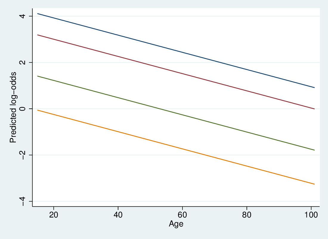
5.2.9 Predicted log odds per contrast
- The predicted log-odds lines are straight and parallel
- The highest relates to the 1-4 vs 5 contrast
- Parallel lines means the effect of a variable is the same across all contrasts
- Exponentiating, this means that the multiplicative effect of a variable is the same on all contrasts: hence "proportional odds"
- This is a key assumption
5.2.10 Predicted probabilities relative to contrasts
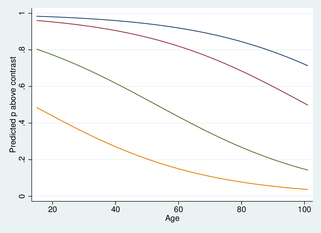
5.2.11 Predicted probabilities relative to contrasts
- We predict the probabilities of being above a particular contrast in the standard way
- Since age has a negative effect, downward sloping sigmoid curves
- Sigmoid curves are also parallel (same shape, shifted left-right)
- We get probabilities for each of the five states by subtraction
5.2.12 Inference
- The key elements of inference are standard: Wald tests and LR tests
- Since there is only one parameter per variable it is more straightforward than MNL
- However, the key assumption of proportional odds (that there is only one parameter per variable) is often wrong.
- The effect of a variable on one contrast may differ from another
- Long and Freese's
SPostStata add-on contains a test for this
5.2.13 Testing proportional odds
- It is possible to fit each contrast as a binary logit
- The
brantcommand does this, and tests that the parameter estimates are the same across the contrast - It needs to use Stata's old-fashioned
xi:prefix to handle categorical variables:
xi: ologit ropfamr i.rsex rage
brant, detail
5.2.14 Brant test output
. brant, detail

Estimated coefficients from j-1 binary regressions

                 y>1         y>2         y>3         y>4
_Irsex_2   1.0198492   .91316651   .76176797    .8150246
    rage  -.02716537  -.03064454  -.03652048  -.04571137
   _cons   3.2067856   2.5225826   1.1214759  -.00985108

Brant Test of Parallel Regression Assumption

    Variable |      chi2   p>chi2    df
-------------+--------------------------
         All |    101.13    0.000     6
-------------+--------------------------
    _Irsex_2 |     15.88    0.001     3
        rage |     81.07    0.000     3
----------------------------------------

A significant test statistic provides evidence that the parallel
regression assumption has been violated.
5.2.15 What to do?
- In this case the assumption is violated for both variables, but looking at the individual estimates, the differences are not big
- It's a big data set (14k cases) so it's easy to find departures from assumptions
- However, the departures can be meaningful. In this case it is worth fitting the "Generalised Ordinal Logit" model
5.2.16 Generalised Ordinal Logit
- This extends the proportional odds model in this fashion
- That is, each variable has a per-contrast parameter
- At the most imparsimonious this is like a reparameterisation of the MNL in ordinal terms
- However, can constrain \(\beta\)s to be constant for some variables
- Get something intermediate, with violations of PO accommodated, but the parsimony of a single parameter where that is acceptable
- Download Richard William's
gologit2to fit this model:
ssc install gologit2
5.3 Sequential logit
5.3.1 Sequential logit
- Different ways of looking at ordinality suit different ordinal
regression formations
- categories arrayed in one (or more) dimension(s):
slogit - categories derived by dividing an unobserved continuum:
ologitetc - categories that represent successive stages: the continuation-ratio model
- categories arrayed in one (or more) dimension(s):
- Where you get to higher stages by passing through lower ones, in which
you could also stay
- Educational qualification: you can only progress to the next stage if you have completed all the previous ones
- Promotion: you can only get to a higher grade by passing through the lower grades
5.3.2 "Continuation ratio" model
- Here the question is, given you reached level \(j\), what is your chance of going further:
- For each level, the sample is anyone in level \(j\) or higher, and the outcome is being in level \(j+1\) or higher
- That is, for each contrast except the lowest, you drop the cases that didn't make it that far
5.3.3 \(J-1\) contrasts again, again different
5.3.4 Fitting CR
- This model implies one equation for each contrast
- Can be fitted by hand by defining outcome variable and subsample for
each contrast (
edhas 4 values):
gen con1 = ed>1
gen con2 = ed>2
replace con2 = . if ed<=1
gen con3 = ed>3
replace con3 = . if ed<=2
logit con1 odoby i.osex
logit con2 odoby i.osex
logit con3 odoby i.osex
5.3.5 seqlogit
- Maarten Buis's
seqlogitdoes it more or less automatically:
seqlogit ed odoby i.osex, tree(1 : 2 3 4 , 2 : 3 4 , 3 : 4 )
- you need to specify the contrasts
- You can impose constraints to make parameters equal across contrasts
6 Special topics: depend on interest
6.1 Alternative specific options
6.1.1 Clogit and the basic idea
- If we have information on the outcomes (e.g., how expensive they are)
but not on the individuals, we can use
clogit
6.1.2 asclogit and practical examples
- If we have information on the outcomes and also on the individuals, we
can use
asclogit, alternative-specific logit - See examples in Long and Freese
6.2 Models for count data
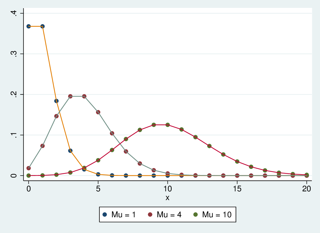
6.2.1 Modelling count data: Poisson distribution
Count data raises other problems:
- Non-negative, integer, open-ended
- Neither a rate nor suitable for a continuous error distribution
- If the mean count is high (e.g., counts of newspaper readership) the normal approximation is good
If the events are independent, with expected value (mean) μ, their distribution is Poisson:
The variance is equal to the mean: also μ
6.2.2 Poisson Density
6.2.3 Poisson regression
- In the GLM framework we can use a regression to predict the mean value, and use the Poisson distribution to account for variation around the predicted value: Poisson regression
- Log link: effects on the count are multiplicative
- Poisson distribution: variation around the predicted count (not log) is Poisson
- In Stata, either
poisson count xvar1 xvar2
or
glm count xvar1 xvar2, link(log) family(poisson)
6.2.4 Over dispersion
- If the variance is higher than predicted, the SEs are not correct
- This may be due to omitted variables
- Or to events which are not independent of each other
- Adding relevant variables can help
6.2.5 Negative binomial regression
- Negative binomial regression is a form of poisson regression that takes an extra parameter to account for overdispersion. If there is no overdispersion, poisson is more efficient
6.2.6 Zero inflated, zero-truncated
- Another issue with count data is the special role of zero
- Sometimes we have zero-inflated data, where there is a subset of the
population which is always zero and a subset which varies (and may be
zero). This means that there are more zeros than poisson would
predict, which will bias its estimates. Zero-inflated poisson (
zip) can take account of this, by modelling the process that leads to the all-zeroes state - Zero-inflated negative binomial (
zinb) is a version that also copes with over dispersion - Zero truncation also arises, for example in data collection schemes
that only see cases with at least one event.
ztpdeals with this.