Next: Quasi-Symmetry Up: Fitting models to square Previous: Fitting models to square
 , that the probability
of changing from
, that the probability
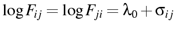
of changing from 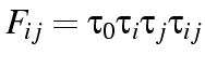 where
where
 and
and
 . One way of fitting this model is
to create a new variable with a different value for each cell in
one half of the table, with the other half of the table being a
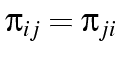
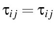
mirror image: that is, for each pair of cells
. One way of fitting this model is
to create a new variable with a different value for each cell in
one half of the table, with the other half of the table being a
mirror image: that is, for each pair of cells
 there is a distinct value of the new variable.
 table the symmetry variable looks like:
| - | 1 | 2 | 3 | 4 | 5 |
| 1 | - | 6 | 7 | 8 | 9 |
| 2 | 6 | - | 10 | 11 | 12 |
| 3 | 7 | 10 | - | 13 | 14 |
| 4 | 8 | 11 | 13 | - | 15 |
| 5 | 9 | 12 | 14 | 15 | - |
tabu VAR1 VAR2 symm .This will lay it out as in the table above.
compute #c=1.
loop #i = 1 to 5.
. loop #j = #i+1 to 5.
.   if var1=#i and var2=#j sym = #c.
.   if var1=#j and var2=#i sym = #c.
.   compute #c=#c+1.
. end loop.
end loop.
if var1=var2 sym=1.
 .
.
 dummy variables, no `real' variable.
 table thus:
compute offdiag = avote<>evote.
makesym avote evote 4 symm .
factor symm s 6.
genlog avote evote with s2 s3 s4 s5 s6
 /cstructure = offdiag
 /print=est/plot=none
 /design= s2 s3 s4 s5 s6
 /save=adjresid.
tabu avote evote adj_1.
 |
| ||||||||