A frequent theme in the medical statistics and epidemiological literature is that odds ratios (ORs) as effect measures for binary outcomes are counter intuitive and an impediment to understanding. Barros and Hirakata (2003), for instance, refer to the relative rate as the “measure of choice” and complain that the OR will “overestimate” the RR as the baseline probability rises. Clearly, ORs are less intuitive than relative rates (RRs), but in this note I take issue with the conclusion sometimes made, that models with relative-rate interpretations should be used instead of logistic regression and other OR models. This is because RRs are not measures of the size of the statistical association between a variable and an outcome since they also vary inversely with the baseline probability), and because, under certain assumptions, ORs and related measures are. That is, RRs may feel more real but they are likely to be misleading.
While the argument is often cast in terms of rejecting logitistic in favour of log-binomial regression and other alternatives, let’s look at some 2*2 tables and hand-calculated ORs and RRs. In the following two tabulations the OR is constant at 2.5, but the baseline probability (in class==0) is respectively 2% and 75%.1
. tab class outcome, matcell(n)

           |        outcome
     class |        No        Yes |     Total
-----------+----------------------+----------
  Class 0  |       980         20 |     1,000
  Class 1  |       951         49 |     1,000
-----------+----------------------+----------
     Total |     1,931         69 |     2,000

. scalar RR = (n[2,2]/(n[2,1]+n[2,2]))/(n[1,2]/(n[1,1]+n[1,2]))
. scalar OR = (n[2,2]/n[2,1])/(n[1,2]/n[1,1])
. scalar D  = n[2,2] - n[1,2]
. di  "RR " %6.3f RR "; OR " %6.3f OR "; N extra outcomes" %5.0f D
RR  2.450; OR  2.525; N extra outcomes   29
|
Here the RR is 2.45, the OR 2.53 and the number of extra outcomes in class 1 is 29, or 2.9%.
           |        outcome
     class |        No        Yes |     Total
-----------+----------------------+----------
  Class 0  |       270        730 |     1,000
  Class 1  |       129        871 |     1,000
-----------+----------------------+----------
     Total |       399      1,601 |     2,000
...
RR  1.193; OR  2.497; N extra outcomes  141
|
But when the baseline probability is high, the RR plummets (suggesting a 19% increase instead of 145%), despite the approximate substantive measure giving 141 or 14.1% extra cases. In this simple case, it seems RRs track substantive significance rather worse than ORs do.
But how do RRs and ORs compare in terms of estimating the size of the underlying statistical or causal association? There are many underlying causal structures possible, but let’s use Stata to simulate a simple one.2 Let the outcome of interest depend on an unobserved (and perhaps unobservable) interval variable. If this propensity is above a certain threshold, the outcome occurs, but let the threshold (and thus the proportion having the outcome) differ from time to time. Let the difference between the two groups be that they have different distributions of the underlying propensity – normal, with the same variance but different means.3 Conceptually, this inter-group difference is the source of effect we are trying to measure, while variation in the threshold is not related to the causal effect. We run the simulation with a sample size of 10,000 and an inter-group difference of 0.2 standard deviations, and 2*2 tables are created for outcome probabilites. Here, for example, for 20% and 60% probabilities:
set obs 10000 gen class = _n <= 5000 gen propensity = invnorm(uniform()) + (class==1)*0.2 sort propensity gen outcome20 = _n > (1 - 0.2)*_N gen outcome60 = _n > (1 - 0.6)*_N |
This yields the following:
           |       outcome20                                  |       outcome60
     class |         0          1 |     Total           class |         0          1 |     Total
-----------+----------------------+----------      -----------+----------------------+----------
         0 |     4,144        856 |     5,000               0 |     2,199      2,801 |     5,000
           |     82.88      17.12 |    100.00                 |     43.98      56.02 |    100.00
-----------+----------------------+----------      -----------+----------------------+----------
         1 |     3,856      1,144 |     5,000               1 |     1,801      3,199 |     5,000
           |     77.12      22.88 |    100.00                 |     36.02      63.98 |    100.00
-----------+----------------------+----------      -----------+----------------------+----------
     Total |     8,000      2,000 |    10,000           Total |     4,000      6,000 |    10,000
           |     80.00      20.00 |    100.00                 |     40.00      60.00 |    100.00

20% probability: RR:  1.34; OR:  1.44              60% probability: RR:  1.14; OR:  1.39
|
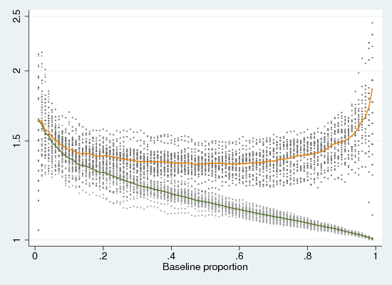
Between 20% and 60% outcome probability, the OR drops but the RR drops rather more. Figure 1 show results for probabilities between 1% and 99%, replicated thirty times (lines or the average values, dots for the actual values). As can be seen, the ORs vary in a shallow U, but the RRs drop precipitously to a zero effect for high baseline probabilities.
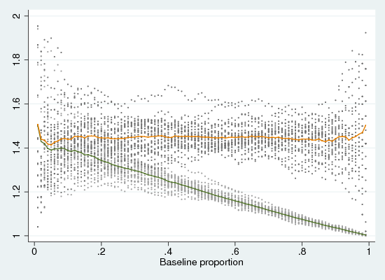
Figure 2 repeats this exercise with logistic rather than normal propensity distributions, with the same variance (logistic distributions resemble normal but have higher kurtosis). Here the average OR is rather more stable. In fact, it can be shown mathematically that the OR is related directly to the difference in means, and is completely independent of the threshold.
Clearly, this causal backstory is simplistic.4 The latent propensity may have other distributions, and the inter-class difference may be other than additive (though, note that log-normal distributions with a multiplicative difference are equivalent in effect to normal with an additive difference). If one class has greater variance, the causal effect will be non-linear (over-represented at both high and low propensity). However, in so far as it is approximately realistic, this story suggests that the odds ratio is a reasonably stable measure of an effect, while the relative rate is superficially intuitive but is not an effect measure.
While the OR and RR can be calculated by hand, the results from logistic (logit outcome class), poisson (poisson outcome class) and log-binomial regression (glm outcome class, link(log) family(binomial)) are exactly the same. The extension to probit regression is obvious. If the simulated distribution is normal, the mean probit estimate (not shown) is as flat as the OR is for the logistic distribution.5
When we are thinking in terms of models, rather than hand-calculated statistics, we can view the propensity distributions as conditional on the other variables. The effect of these variables is analogous to shifting the threshold. In this case, the RR will be unreliable even if the average level of the outcome is stable, if there are other variables with large effects on the outcome. Thus, unless predicted probabilities in the data are all very low (say, under 10%) it seems unwise to base interpretations on RR models. If it is important for the audience to see effects on probabilities, use -margins- to report marginal effects for different configurations of covariates. The fact that marginal effects vary with the values of the covariates is a feature, not a bug, reflecting the complexity of reality rather than being a wrong-headed consequence of an awkward model.
Bibliography
Barros, A. J. and Hirakata, V. N. (2003).- Alternatives for logistic regression in cross-sectional studies: An
empirical comparison of models that directly estimate the prevalence ratio.BMC Medical Research Methodology, 3(21).
Footnotes
- … 75\%.1
- Stata
code at http://teaching.sociology.ul.ie/catdat/ortab.do. - …
one.2 - Stata code at
http://teaching.sociology.ul.ie/catdat/orsim.do. - …
means.3 - The attentive reader may recognise this as related to
the latent variable justification of the logistic regression model,
but for the moment please consider its plausibility as a simple causal
model. - … simplistic.4
- It also suits
only one-off outcomes – if the outcome is a result of exposure over
time, the OR is as misleading as the RR, and an estimate of the
hazard-rate ratio is needed. - …
distribution.5 - If you multiply the probit estimate by pi/sqrt(3), it approximates the log of the odds ratio quite closely.

