Logit vs LPM with differing ranges of observation of X
The linear probability model (LPM) is increasingly being recommended as a robust alternative to the shortcomings of logistic regression. (See Jake Westfall’s blog for a good summary of some of the arguments, from a pro-logistic point of view.) However, while the LPM may be more robust in some senses, it is well-known that it does not deal with the fact that probability is restricted to the 0–1 range. This is not just a technical problem: as a result its estimates will differ if the range of X differs, even when the underlying process generating the data is the same. For instance, if X makes the outcome more likely, and we observe a moderate range of X we will get a certain positive slope coefficient from the LPM. If we supplement the sample with observations from a higher range of X (sufficiently high that the observed proportion with the outcome is close to 100%), the slope coefficient will tend to be depressed, necessarily to accommodate the observations with the higher X but the at-most marginally higher proportion of the outcome. The same is not true of the logistic model.
(I have already blogged about inconsistencies in the LPM in the face of changes in the data generating process; here, I am talking about inconsistencies of the LPM where the observed range of X changes under an unchanging data generation model.)
In other words, if there are different sub-populations where the true relationship between X and the outcome is the same, but the range of X is different, the LPM will give less consistent results than the logistic regression model.
We can demonstrate this by generating data over wide range of X, and fitting models on truncated data sets. We use a latent variable that depends on X:
y* = -5 + x + N(0,2)
and define the outcome as \(y = y*>0\). For the purposes of the example, X is given a uniform distribution between 0 and 10.
We use Stata to implement this:
set obs 5000
gen x = runiform()*10
gen ystar = -5 + 1*x + rnormal(2)
gen y = ystar>0
lowess y x, bw(.125)
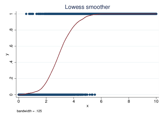
Figure 1: Lowess, latent propensity data generation
Lowess provides a non-parametric summary of the relationship between X and the outcome (see Fig 1). This shows an intuitively attractive summary of the relationship between X and Y. At low levels of X, the prediction is near zero, and then it starts to rise gently, then faster, and then as it approaches one it slows its rise and reaches (and follows) a ceiling of one. (Admittedly, the very good match between the lowess curve and the classic “sigmoid curve” of logistic regression is due to using the latent propensity variable to relate X to the outcome, but any reasonable model that relates X to the closed probability interval is going to share these broad characteristics. See also section 2.)
The slope coefficients from logit and LPM models are not directly comparable. However, we can compare their predicted probabilities, and examine how that changes when exposed to different subsets of the data set. We do this by fitting successive models for X <= 1, X <= 2, up to X <= 10 (i.e., finally the full data).
forvalues x = 1/10 {
  su y if x<=`x'
  if (r(min)<r(max)) { // check that both yes and no outcomes are observed
    reg y x if x<=`x'
    predict lpm`x' if e(sample)
    logit y x if x<=`x'
    predict log`x' if e(sample)
  }
}
For each model, we generate predicted values for the truncated range, and graph these:
scatter y x || ///
  scatter lpm* x, ///
  msize(.2 .2 .2 .2 .2 .2 .2 .2 .2 .2) ///
  legend(off) name(gr1, replace) title("LPM")
scatter y x || ///
  scatter log* x, ///
  msize(.2 .2 .2 .2 .2 .2 .2 .2 .2 .2) ///
  legend(off) name(gr2, replace) title("Logit")

graph combine gr1 gr2, xsize(8) ysize(3) iscale(*1.5)
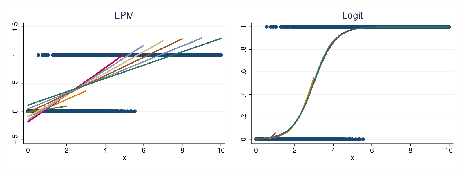
Figure 2: LPM and logistic results, latent propensity data generation model
As we can see from the graphs in Fig 2, neither model is very consistent when we observe only very low ranges of X, but for X <= 4 and higher, the LPM gives a systematic pattern of decreasing slopes, agreeing with the expectation proposed above. However, the logistic regression gives results that are almost entirely self-consistent.
Other models of data generation
The data generation model above is very congenial to logit. In fact, it directly implies the probit model, in that the implicit relationship between X and the probability of the outcome is the normal CDF (in practice, logit and probit differ very little). What if the data generating model is radically different?
In this section we re-run the analysis with a non-continuous model. For values of X between 3 and 6 the probability of the outcome rises linearly from 0.01 to 0.99. Outside that range it is either 0.01 (X<3) or 0.99 (X>6). (The probability range is from 0.01 to 0.99 in order for the data to be indeterministic.)
P(y=1) = min(0.99,max(0.01, (x-3)/3))
This is a quite unrealistic model, but it fulfills (if by brute force) the criterion that P must be bounded between zero and one, and it does so without making any of the assumptions about the distribution of a latent propensity that the logit and probit models do.
clear
set obs 5000
gen x = runiform()*10
gen p = min(0.99,max(0.01, (x-3)/3))
gen px = runiform()
gen y = p>px
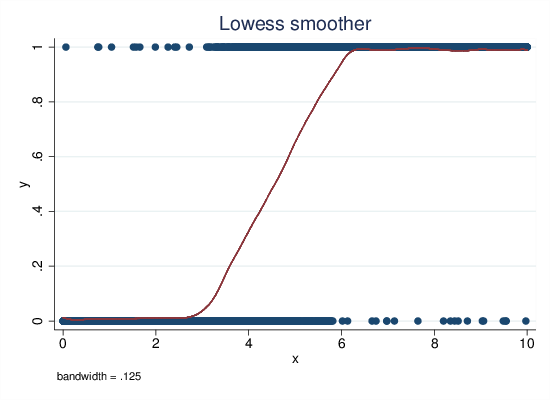
Figure 3: Lowess, non-continuous data generation
The lowess plot in Fig 3 captures the data generating model quite well (but naturally, it does not reproduce the sharp kinks at X=3 and X=6).
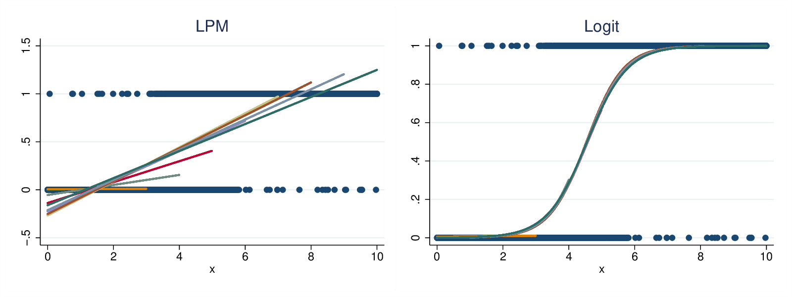
Figure 4: LPM and logistic results, non-continuous data generation model
The LPM slopes start low, strongly affected by the zero slope for X<3 when looking at X<=4, but then start rising, until the zero slope for X>6 starts to reduce the slope again. The logistic model is also more inconsistent than in the first example, particularly with very truncated data. For X<=4 the slope is clearly biased up. However, when given fuller ranges of the data it quickly becomes more self-consistent. (Note that data sets of X<=3 and below both models should give a zero slope as in that range the outcome is independent of X.)
So even with this data generating process that is not directly congenial to logit, the bounded range of the probability means that the logit model gives much more consistent results than the LPM.
Logit vs Probit
The similarity between logit and probit has been mentioned in passing. The first data generating model corresponds directly with the probit model. Let’s quickly compare logit and probit under the two data generation processes.
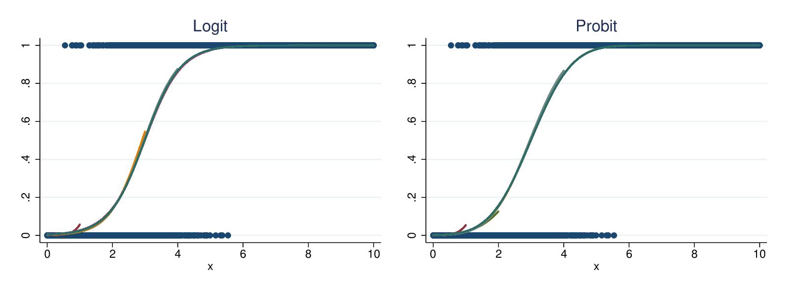
Figure 5: Logit vs Probit, continuous data
Fig 5 shows the predict probabilities under the first data generation model. The curves are very similar in their values, and their self-consistency.
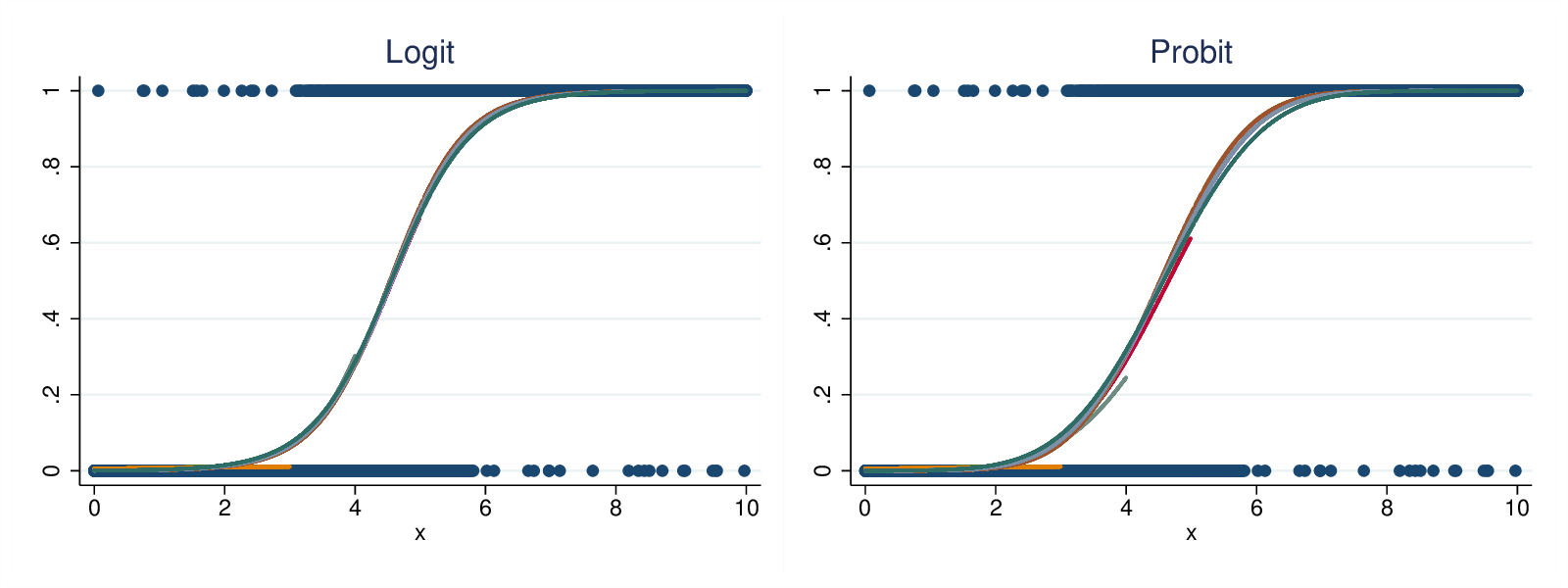
Figure 6: Logit vs Probit, non-continuous data
Fig 6 shows the predicted probabilities under the second data generation model. Again the curves are very similar (though the logit curves are marginally more self-consistent). Thus we can argue that the advantages of the logit model over the LPM apply equally to the probit model.
Conclusion
Whatever the data generating structure, probability is bounded. As X increases, the propensity to have the outcome cannot exceed 1. Whether this is by a clipping or a smooth s-shaped function, the logistic and probit models do better than the linear probability model, when we extend the range of observation to include more high values of X with their concomitant high propensities to have the outcome. Logit and probit coefficients remain relatively stable, while the linear probability model responds to the extra cases by reducing the estimated slope. We can quibble with the functional form implied by the logistic and probit models (i.e., whether in reality there is a latent propensity with a normal or logistic distribution), but they (at least approximately) solve the problem caused by the bounded nature of the probability of a binary outcome, whereas the LPM does not.
In short, for a given data generation structure, the LPM is more sensitive to sampling extra cases at the high (or, by symmetry, the low) end. If we have two sub-populations where the underlying model is the same, but one has a wider range of X, the LPM may give inconsistent results across the sub-populations, whereas the logistic and probit models will be more robust.
This matters only when you add cases with very high values of X (such that their prediction under the existing LPM model would be in excess of one, or their prediction under the logistic model very near to one), or (by symmetry) very low values of X. That is, however, just another way of expressing the common advice that the LPM performs well as long as the predicted probabilities fall in the range 0.2 to 0.8. If you have values outside that range, you are risking underestimating the effect with the LPM but not with the logistic and probit models.