One of the key anxieties about sequence analysis is how to set substitution costs. Many criticisms of optimal matching focus on the fact that we have no theory or method for assigning substitution costs (Larry Wu’s 2000 SMR paper is a case in point). Sometimes analysts opt for using transition-probability-derived costs to avoid the issue.

My stock line is that substitution costs should describe the relationships between states in the basic state space (e.g., employment status), and that the distance-measure algorithm simply maps an understanding of the basic state-space onto the state-space of the trajectories (e.g., work-life careers). Not everyone finds this very convincing, however.

I’ve been playing recently with a set of tools for evaluating different distance measures, and it struck me that I could use them to address this issue. Rather than compare hand-composed substitution matrices, however, I felt an automated approach was needed: randomise the matrices, and see what the results looked like. Can we improve on the analysts’ judgement? What are the characteristics of “good” substitution cost matrices?

This gave two problems: how to randomise matrices, and how to judge effectiveness. The latter problem I sorted by defining effectiveness as the ability to predict a covariate of the trajectory, operationalised as the statistical test comparing a model with as RHS variables only simple summaries of the trajectory (start and end values, and cumulated duration in each state) with one that additionally included seven dummies for an eight-category cluster solution based on the distance measure. Given a binary covariate (for instance, whether attended grammar school, using the McVicar-Anyadike Danes data), the “score” is represented by the likelihood-ratio chi-sq. Testing it against simple summaries of the trajectory makes sure that the sequence analysis is giving real added value, and not simply picking up crude characteristics.

Randomising the substitution cost matrix was a little more complicated. Generating a triangle of random values (and its mirror image) doesn’t work, because that will infringe the triangle inequality as often as not, and the optimal matching algorithm yields metric distances only when the substitution costs imply a metric space. The best solution there seemed rather to randomise the location of the states in a virtual Euclidean space, and to derive the distances from their coordinates. For m states you need at most m-1 dimensions. This can be done in a few lines of Mata, Stata’s matrix language.

From there, using Stata’s postfile system (ask, if you’d like to see the code), it is fairly easy to collect results for a large number of runs, matching the substitution matrix with an indel cost of half the maximum substitution cost. Luckily, the plugin-based oma command is fairly quick, so 1,000 runs takes perhaps 15 hours (on an elderly PC).

So what do the results look like? For comparison, the test using Duncan McVicar and Michael Anyadike-Danes’ published substitution costs give a likelihood-ratio statistic of 40.98 (7 df, p<0.001). That is, there is a strong association between having attended grammar school and the 8-group cluster solution, even after controlling for the basic trajectory characteristics.

Here is a histogram of the LR-test statistic for 1,000 runs:

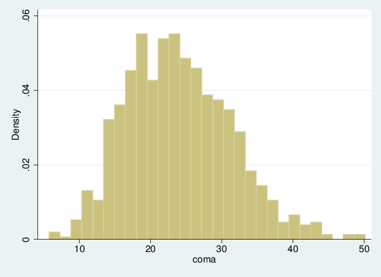
As we can see, for this specific test, the MVAD costs do quite well: only about 2.5% of random cost structures do better. Clearly for other variables the results are likely to differ, and this sort of test is not necessarily the definitive scale by which to judge sequence analysis, but it does show that the analysts’ judgement worked well in this case.

There’s more to get out of this analysis, in particular to look at the relationship between the substitution costs and the outcome (and here the results are less encouraging), but that’s enough for one blog post.