How well does multi-seat constituency STV select candidates?
Multi-seat STV as a voting system is meant to yield approximately proportional outcomes (parties proportions of seats should approximate their proportion of the vote). It has other advantages, primarily that voters don’t need to vote tactically, since their preferences will be reflected (if your favourite candidate has no hope, voting for them is not throwing away your vote). But compared with other ways of electing people in multi-seat consitituencies, how well does it perform?
“Well” is hard to define. One way of thinking about it would be in terms of the distance between each voter and their nearest elected candidate. A system that maximises the closeness of each voter to the nearest candidate can be regarded as desirable. However, we can’t assess this empirically without a lot of onerous data collection. But what if we simulate? I’ve written a small simulation of the STV process, that assigns candidates and voters positions on two dimensions (see Figure 1), and derives voters’ preferences from the resulting Euclidean distances (plus a random disturbance). We can assess the “fit” of the elected candidates by calculating the average distance of each voter to the nearest candidate.
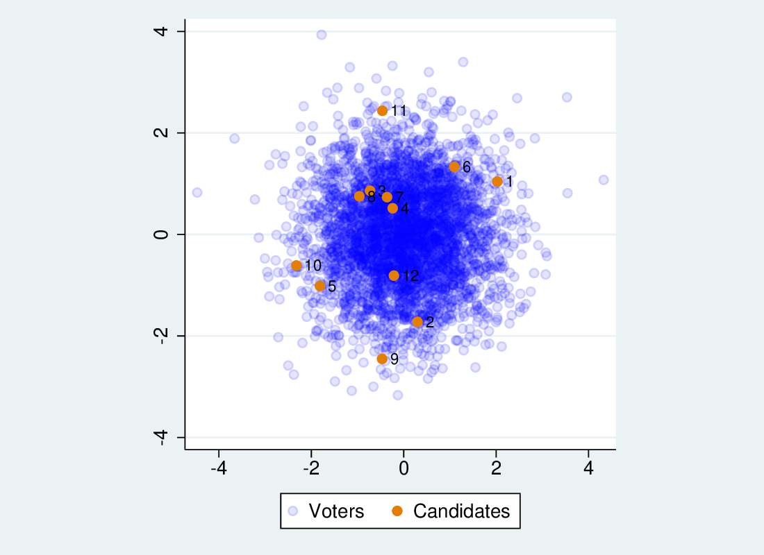
Figure 1: Simulated voters and candidates on two dimensions
I compare 3 methods: STV; counting 1st preferences only and electing the first N candidates (where N is the number of seats); and treating the first N preferences as votes for each of the N seats. In the last method, we simply count each of the first N preferences equally, pooling them and electing the resulting top candidates. Each method yields a combination of the candidates, probably different. In order to get an idea of how close each method gets to the best possible combination, I also calculate the fit for all possible combinations of candidates): the optimal candidates.
See Figure 2 for an example output from the simulation. Candidates 4, 6 and 12 are elected by both first preference and STV, and are also part of the optimal combination. STV’s 4th candidate is optimal, but not the other first preference candidate (the first N preferences outcome is not shown).
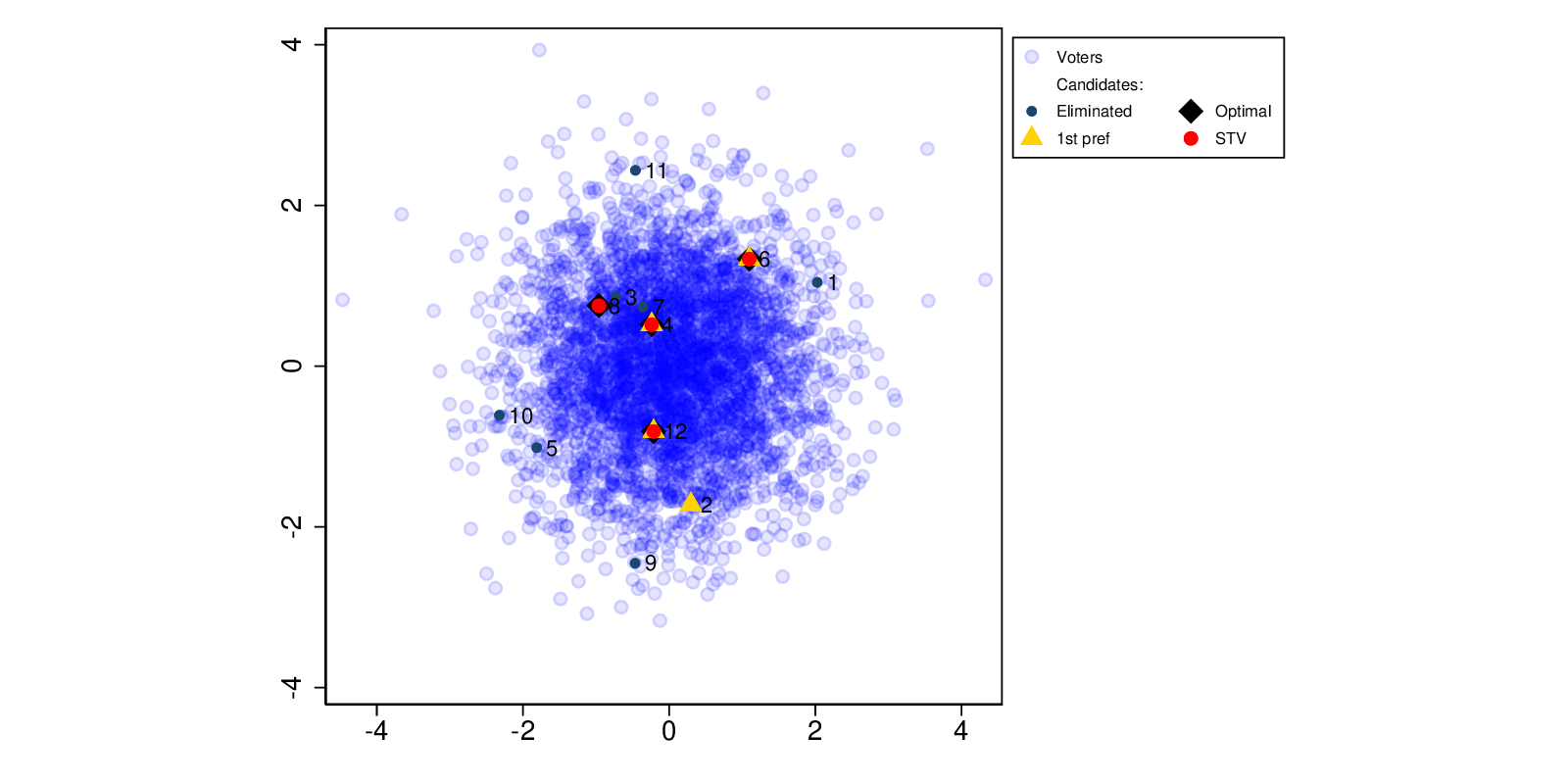
Figure 2: Simulated election: STV, first preference and optimal.
We run the simulation 10,000 times to get a stable estimate of the average result. The simulation has 12 candidates in a 4-seat constituency, and 4,000 voters. Voters and candidates are distributed similarly (bivariate normal, with the same mean and variance). That is, there is no voter polarisation, and there is no sort of voter that is particularly disadvantaged with respect to candidates (as there would be if candidates were, for instance, on average to the right of voters). See Figure 1 again.
This gives the following mean average distance to nearest candidate:
| Method | Average distance to nearest candidate |
|---|---|
| STV | 0.959 |
| First preference | 0.983 |
| Pool first N preferences | 1.057 |
| Optimal combination | 0.928 |
STV gives a clearly better result on average than first preference, but doesn’t on average achieve as good a score as the optimal choice. Nonetheless, STV often picks the optimal combination, as does first preference (but less often than STV). Pooling the first N preferences gives the poorest result: this is not surprising as it is throwing away preference information within the first N. It selects candidates that are disproportionately close to the centre.
So in the absence of polarisation, where the distribution of candidates more or less matches that of voters, STV performs better than first preference or first N preference voting. It doesn’t automatically yield the best possible result, however.
Truncated preferences
In the simulation above, all voters voted all the way down the ballot. What happens to the efficiency of STV if voters may give up part way? It’s a hard task to rank high numbers of candidates, and in real life many or most voters do not complete the ballot, stopping for instances after three or four preferences.
I re-run the simulation, imposing a random truncation on the preference list. That is, at random voters mark between 1 and 12 preferences. Again running 10,000 simulations yields the following data:
| Method | Full ballot | Short ballot |
|---|---|---|
| STV | 0.959 | 0.953 |
| First preference | 0.983 | 0.983 |
| Optimal combination | 0.928 | 0.928 |
Results for first preference and the optimal combination do not change materially (they are not affected by the change), but the result for STV slightly improves. Incomplete ballots don’t seem to be a problem, and don’t reduce the efficiency of STV. This is a surprise: I expected to see a small degradation. The absence of a disimprovement however does chime in with earlier explorations I did with the simulation that demonstrated that later preferences come in to play at a rapidly declining rate. As Figure 3, in a 12-candidate/4-seat constituency, preferences beyond about the fifth rarely come into play.
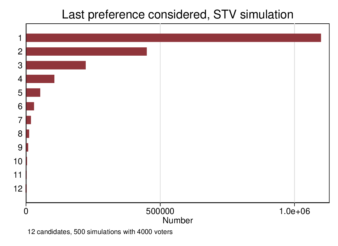
Figure 3: What’s the lowest preference that matters?
Conclusion
On the evidence of this simulation (which is of course not the real world), STV yields good results on the metric we have considered: how close each voter is to the nearest elected candidate. It yields better results on average than just considering first preferences, and considering first N preferences does poorly. Moreover, voters not completing the ballot does not seem to have a negative effect on the efficiency.
Experiments not reported here suggest that these conclusions may be modified if we allow for voter polarisation or a mismatch between voters and candidates: unfortunately, exploring simulation parameter spaces takes a lot of time.