Category Archives: Stata

The shortest day and the earliest sunset

Everyone knows that Midwinter’s Day, the day of the Winter Solstice, is the shortest day of the year. I think about this a lot, mostly every December/March/June/September (also around DST time changes). A few years ago I discovered the R “suncalc” package. It’s full of interesting astronomical functions, and can show the timing of sunrise, sunset, solar noon and a whole lot of other things, for any date and location. So I’ve been playing with it to help me understand what’s going on.

library(suncalc)
library(ggplot2)
data = getSunlightTimes(date = as.Date(seq(0,32), origin="2023-12-08"), lat=52.7, lon=-8.6)
data$daylength = data$sunset - data$sunrise
ggplot() + geom_point(data=data, aes(x=as.Date(sunrise), y=daylength))

daylength.png

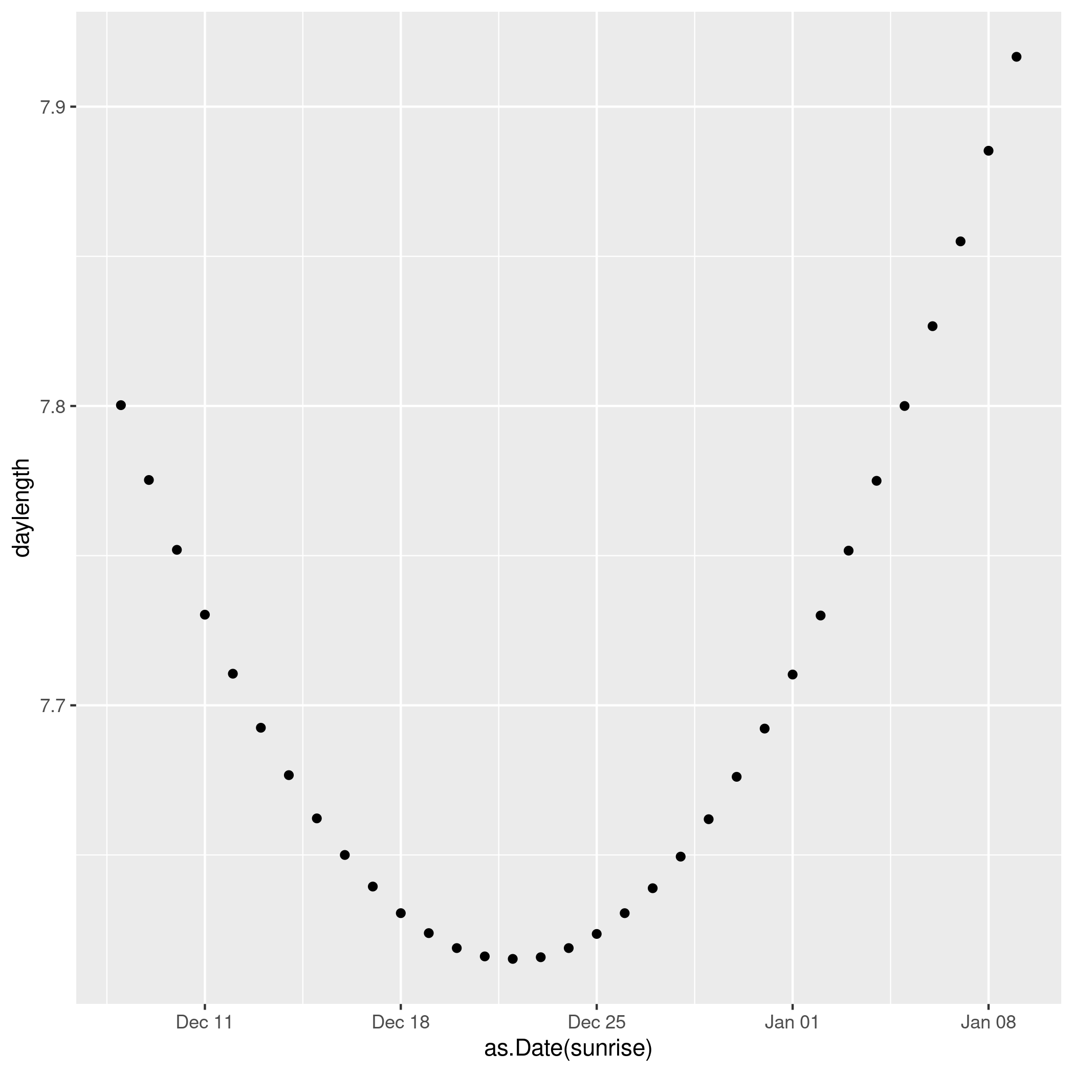
We see clearly that the shortest day in 2023 was Dec 22 (the exact solstice moment was 22 Dec, 03:27).

But the earliest sunset doesn’t actually happen then. It actually happened a few days earlier, Dec 15.

Continue reading The shortest day and the earliest sunset

SDMKSUBS: A new SADI command for substitution costs

A new command

In this blog I introduce a new utility command, sdmksubs, which creates substitution cost matrices for sequence analysis, as part of the SADI Stata add-ons.

Most sequence-analysis distance commands require the specification of substitution costs, which describe the pattern of differences in the state space through which the sequences move. These can be derived from theory, from external data, or can be imposed by researcher fiat. It is also common to use the pattern of transitions in the sequence data to derive them, though this is not an unproblematically good idea. The existing trans2subs command in SADI calculates simple transition-based substitution costs. The new sdmksubs calculates this substitution cost structure, and a range of others, some simple “theoretical” ones, and some based on the transition pattern, but taking more of the data into account than the traditional trans2subs matrix.

SADI is a Stata package sequence analysis of data such as lifecourse histories, and has been around for quite a while. Recent improvements includes fixes for internal changes in Stata 18, lifting limits on sequence length, etc., but here I focus on sdmksubs only.

Continue reading SDMKSUBS: A new SADI command for substitution costs

Three-way referendums: Condorcet vs Instant Runoff

Simulating 3-way choice

I’ve been thinking about a potential second Brexit referendum, where a three-option menu is given:

  • 1: Exit the EU with no deal
  • 2: Accept the negotiated deal
  • 3: Remain in the EU

Three-way choices are alien to British experience of referendums, but don’t really pose great difficulties. First Past The Post (FPTP) is clearly undesirable, but instant runoff (IRV) and Condorcet voting are easy to implement and explain to the electorate. So I built a little simulation to help me understand the problem, particularly to look at the relative performance of IRV and Condorcet.

My conclusions in brief: Condorcet is much more likely to go for the compromise solution (the deal), IRV less so and FPTP the least. Condorcet also seems to correspond well with the average of the underlying utilities. When the population is skewed pro-leave or pro-remain, IRV and Condorcet give more similar results (because it becomes more of a two-horse race). Condorcet cycles are rare. Finally, FPTP is crap.

Continue reading Three-way referendums: Condorcet vs Instant Runoff

Comparative perspective on migration from Eurostat population data

Migration is a big issue at the moment in Europe, not least in the UK
where public fears about migration (stoked by a racist press and a Home
Secretary and now PM who, let’s say, seems to have a visceral unreasoned
belief that the presence of foreigners in some way harms Britain) lie
behind the Brexit vote.

There are other reasons for being interested in migration, of course.
For instance, I’ve been wondering a bit about gender differentials in the age profile
of migration and re-migration. So I started looking for data, initially
on the Irish CSO site, where I found annual year-of-age
population estimates.

Continue reading Comparative perspective on migration from Eurostat population data

UCAS, ethnicity and admission rates

UCAS, the UK university admissions clearing house, have released data relating to ethnicity and admissions to English universities, in part in response to Vikki Boliver‘s research in Sociology suggesting that members of ethnic minorities are less likely to be admitted to Russell Group universities.

The analysis note with the release is sober and correct, showing a mostly consistent pattern of offer rates for ethnic minority students being lower (but not far lower) than expected. However, UCAS’s press release seems to have suggested that the effect is almost explained away, and attributes it to ethnic minority students disproportionately applying to courses with low acceptance rates. This does not seem to be the case.

Update: see also next blog entry.
Continue reading UCAS, ethnicity and admission rates

Mapping with Python and Stata

Elevation data for large swathes of the planet have been collected by NASA and are available to download from http://dds.cr.usgs.gov/srtm/.

The data is contained in binary files, each representing a 1-degree by 1-degree “square”. Here are five lines of Python and four lines of Stata that will turn the data into a simple graph:

import struct
file = open("data/N52W011.hgt", "r")
for y in range(1201):
for x in range(1201):
print y, x, struct.unpack(">h",file.read(2))[0]

Do python file.py > map.dat. Then run this Stata code:

infile i j height using /tmp/ext.dat
gen h2 = int(sqrt(height))
replace h2 = 30 if h2<=0
hmap j i h2, nosc

Low res version of map

(Hi-res version.)

You may need to install Python’s struct package, and Stata’s hmap add on, but they’re available from the usual locations.

There are better ways of doing this, of course: it’s slow, the aspect ratio is wrong, the colours are not ideal and the axis labelling is bad. Even worse, it is a complete abuse of the hmap add-on. It’s a quick and dirty way to turn binary data into pictures, all the same.

Discrepancy analysis in Stata

In Studer et al (2011) an important new tool is introduced to the field of sequence analysis, the idea of “discrepancy” as a way of analysing pairwise distances. This quantity is shown to be analogous to variance, and is thus amenable to ANOVA-type analysis, which means it is a very attractive complement to cluster analysis of distance matrices.

This has been implemented in TraMineR (under R), along with a raft of other innovations coming out of Geneva and Lausanne. Up to now it hasn’t been available elsewhere. I spoke to Matthias Studer at the LaCOSA conference, and he convinced me that it was easy to code, and that all the information required was in the paper. This turned out to be the case, and I have written an initial Stata implementation. Continue reading Discrepancy analysis in Stata

Cluster analysis is unstable, we knew that!

Experience tells me that small changes in the data can lead to substantial changes in the solution of a cluster analysis. This is especially true when the space is sparsely populated, as is the case with sequence analysis of lifecourses. Small changes in parameterisation (e.g., substitution costs) can lead to substantial differences in the cluster solution.

However, recently I came across an extreme case of sensitivity. Continue reading Cluster analysis is unstable, we knew that!

Tips for Stata console mode

There are really three main ways of interacting with Stata:

  • In batch mode
  • Console mode
  • Through the GUI

Batch mode is critical to reproducible, self-documenting code. Even if you don’t use it, its existence is a reflection of the idea of a single do-file that takes you from data to results in a single movement. Most people use Stata through the GUI, most of the time, though, even when their goal is a pristine goal-oriented do-file. Stata’s GUI is clean, efficient and pleasant to use.

Console mode, on the other hand, is like the dark ages: a text mode interface (reminiscent of the bad old days before Windows 3.1, of DOS and mainframes). Why would anyone use it? Continue reading Tips for Stata console mode

Substitution costs in sequence analysis — randomise!

One of the key anxieties about sequence analysis is how to set substitution costs. Many criticisms of optimal matching focus on the fact that we have no theory or method for assigning substitution costs (Larry Wu’s 2000 SMR paper is a case in point). Sometimes analysts opt for using transition-probability-derived costs to avoid the issue.

My stock line is that substitution costs should describe the relationships between states in the basic state space (e.g., employment status), and that the distance-measure algorithm simply maps an understanding of the basic state-space onto the state-space of the trajectories (e.g., work-life careers). Not everyone finds this very convincing, however.

I’ve been playing recently with a set of tools for evaluating different distance measures, and it struck me that I could use them to address this issue. Rather than compare hand-composed substitution matrices, however, I felt an automated approach was needed: randomise the matrices, and see what the results looked like. Can we improve on the analysts’ judgement? What are the characteristics of “good” substitution cost matrices?

Continue reading Substitution costs in sequence analysis — randomise!