When we have a binary outcome and want to fit a regression model,
fitting a linear regression with the binary outcome (the so called Linear
Probability Model) is deprecated, and logistic and probit regression are
the standard practice.

But how well or poorly does the linear probability model function
relative to logistic or probit regression?

We can test this with simulation. Let’s assume the outcome is affected
by one continuous variable, X1, and one binary variable, X2, and focus
on the estimate of the effect of X2. Let’s also assume that the data
generating process is well described by the latent variable model of
binary regression: we assume an unobserved variable Y* which has a
simple linear relationship to two explanatory variables, X1 which is
continuous, and X2 which is binary. Consider Y* as the propensity to
have the outcome: if Y* is above a threshold, the variable Y is observed
to be 1, otherwise 0.

gen ystar = 0.5*x1 + 0.2*x2 + rnormal()
gen y = ystar > `threshold'

Let’s focus on the effect of X2, the binary RHS variable. We can think
of this as a group difference: X2 == 1 means a higher Y* for any given
level of X1, but the underlying propensity has the same distribution
(just a higher mean). In particular, what happens to the estimate of the
effect of X2 as the threshold varies? Is the estimate consistent as the
outcome varies from rare, to common, to almost universal?

I create a simulation, N=1000, where Y* and Y are defined as above, but
set the threshold repeatedly, such that Y==1 varies from 1% to 99%. In
each case I run a linear probability model, a logit and a probit:

reg y x1 i.x2
logit y x1 i.x2
probit y x1 i.x2

Running this 100 times generates the following graph:

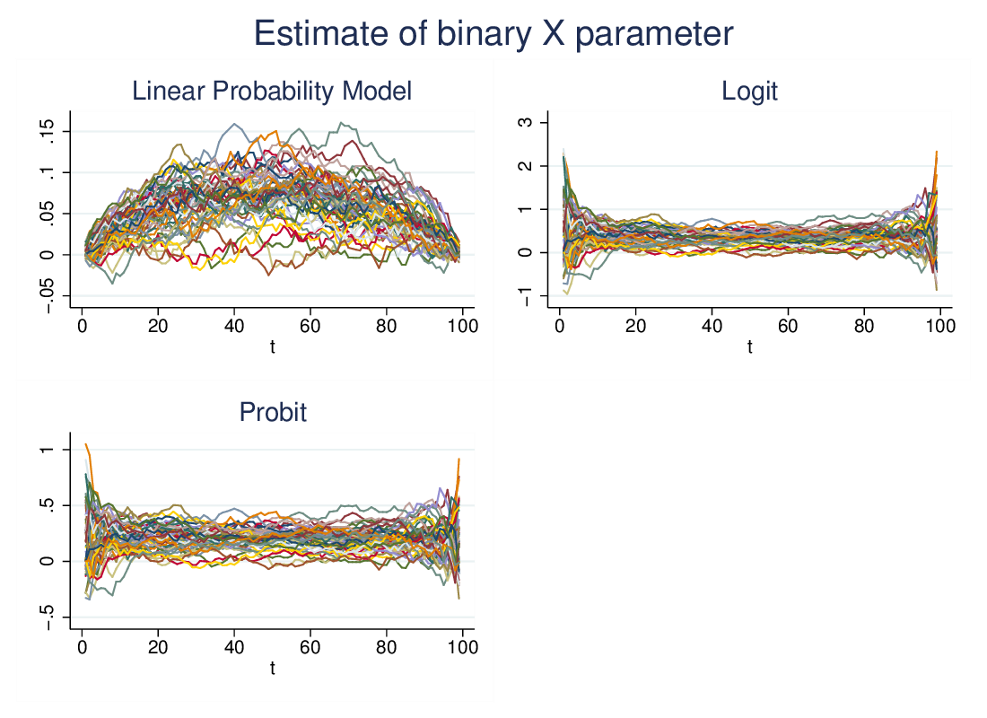
Both logit and probit are quite inconsistent in the extremes, where
either Y==1 or Y==0 is very rare, but give consistent estimates in the
bulk of the range. LPM however generates estimates which are strongly
affected by the threshold, tending to zero at the extremes and to a maximum
near 50%. In other words, though the real effect of the binary X
variable is constant, the LPM reports an estimate that is also affected
by the distribution of the Y outcome variable.

This perspective on the latent variable model of binary outcome
generation is also illustrated in interactive form at
http://teaching.sociology.ul.ie:3838/apps/orrr/. In that app there are
two groups with the same distribution of a propensity to have a
particular outcome, but with a settable difference in means (top slider)
and a settable threshold (bottom slider). For a given difference in
means, it will be seen that the odds ratio is relatively stable when the
underlying distribution is normal, and a constant when the distribution
is logistic (the distribution can be selected below the sliders).
However, the difference in proportion varies widely, near zero when the
cutoff is very high or very low, and at a maximum near the middle
(actually when the cutoff is at the point the distribution lines cross).
(The logistic regression with standard deviation 1/1.6 is similar in
shape to the standard normal distribution, but has different
mathematical properties.)

The logistic regression binary parameter is in fact the log of the odds
ratio, making the assumption that the underlying distribution is
logistic. The probit parameter relates analogously to the normal
distribution (the main difference is scale). However, the Linear
Probability Model’s parameter is related to the difference in
proprortions.

Thus we see from two angles that, given the latent variable picture is a
good model of the data generation process, that “sigmoid curve”
approaches like logistic and probit regression are distinctly better
than the linear approximation.

Reality is likely more complicated than the simple latent variable
model. For instance, there may be heteroscedasticity such that the
variance of the propensity varies with X1 and/or X2. However, it’s a
good starting point.