In an idle moment this afternoon, I wrote a Stata command.

It was to create a light-weight implemention of the “percentogram” described at https://statmodeling.stat.columbia.edu/2023/04/13/the-percentogram-a-histogram-binned-by-percentages-of-the-cumulative-distribution-rather-than-using-fixed-bin-widths/, and I like the result, but it struck me that it is a good example of how practical and useful it can be to engage in Stata programming. Also, it’s a good example of how writing code in Stata (in a programmable command language) is very different from writing code in a stats-capable programming language like R, Python or Julia.

It’s easy to code a Stata command. All you need is a Stata program, say xyz, in a file xyz.ado in a location that Stata sees (check out Stata’s adopath). And thanks to the syntax command, and various ways of passing options, it’s easy to write a command with flexible and complex invocations, just like real Stata commands.

The key things this example demonstrates are

• how ado-files work
• the powerful syntax command
• the flexible and powerful local macro system
• how Stata commands leave results behind them for other commands to use (return)
• how commands can access a lot of the power of the other commands they invoke (e.g., with the asterisk option)
• and a little bit about how the new frames system works

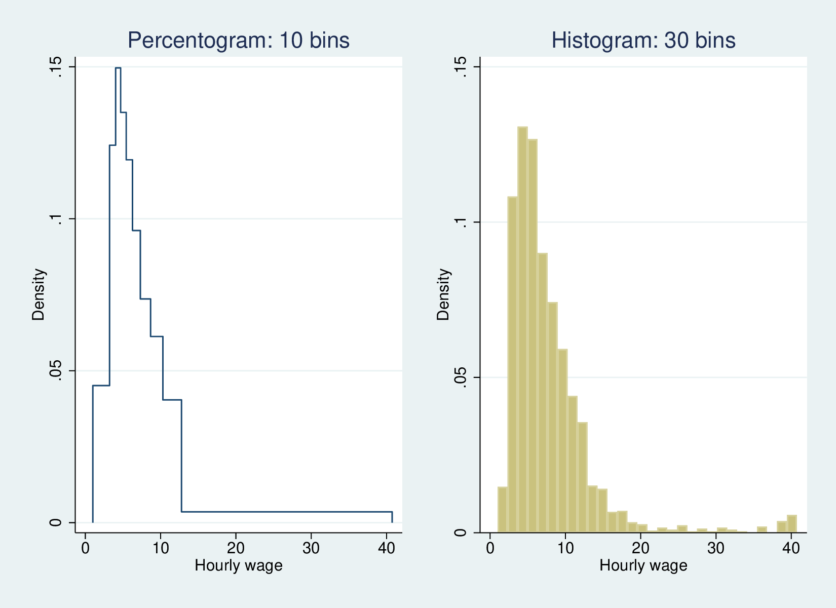
First, let’s look at what it does:

sysuse nlsw88
percentogram wage, bins(10) title("Percentogram: 10 bins") name(gr1, replace)
histogram wage, bin(30) title("Histogram: 30 bins") name(gr2, replace)
graph combine gr1 gr2

Now, let’s look at the complete code, the contents of percentogram.ado

program percentogram
version 16.0
syntax varlist(min=1 max=1), BINs(integer) *
local nb = `bins'+2
local vl : var label `varlist'
quietly {
  centile `varlist', centile(0(`=100/`bins'')100)
  tempname fr
  frame create `fr'
  frame `fr' {
    set obs `nb'
    gen x = .
    label var x "`vl'"
    forvalues i = 1/`=`nb'-1' {
      replace x = r(c_`i') in `i'
    }
    gen d = 1/((x - x[_n-1])*(`bins'))
    label var d "Density"
    replace d = 0 in 1
    replace d = 0 in `nb'
    replace x = x[_n-1] in `nb'
    line d x, connect(step) `options'
  }
}
end                

The first really powerful command is syntax. This is the command that handles passing variable names and options to all Stata commands, and is enormously flexible. Here, it tells the command to expect exactly one variable name, and a required option bins which takes a numeric parameter. The asterisk allows special treatment of any other options (more below). This allows the command to be invoked like this:

The program runs from program percentogram to the corresponding end. It has a version 16.0 statement to say it will work on this version or any later (the frames facility was introduced in version 16).

. percentogram wage, bins(10)

Stata’s language is a command language, not a full programming language. It uses macros (local and global) as the main form of working variable, but it has a good range of flow controls, conditionals. Global macros ($ABC) are persistent, but local macros (`ABC') are more useful (and ephemeral). They are evaluated using the `' pair. The syntax command makes the variable list available in the macro varlist and the “bins()” option as the macro bins. The first thing the body of the program does is create another local macro, nb, which is the number of bins plus 2, with local nb = `bins'+2. The next command shows another aspect of local variables: they can access all sorts of other information. The line local vl : var label `varlist' simply extracts the variable label of the single variable in the varlist macro. See help local in Stata for an overview, and help extended_fcn on how macros can extract all sorts of info from Stata.

The remainder of the program is wrapped in a quietly{} block: this suppresses output. The first bit of suppressed output is that of the centile command, which does the work of determining the quantiles. The argument to the centile() option uses Stata range notation: 0(10)30 would evaluate to 0 10 20 30. The actual code, 0(`=100/`bins'')100 demonstrates another aspect of local macros: on the fly evaluation. Where Stata expects a number, and not an expression, a macro invocation of the form `=…' will do the evaluation in place. `=100/`bins'' is 100 divided by the required number of bins.

Let’s ignore the tempname and frame commands for a moment, and we’ll see how Stata programs access information from other programs. Normally (without the quietly prefix) the centile command prints the relevant information to the screen:

sysuse nlsw88
centile wage, centile(0(20)100)

What it also does is post a lot of results to where they can be accessed by the macro infrastructure

sysuse nlsw88
qui centile wage, centile(0(20)100)
return list

We can access individual elements like r(c_1). Having initialised a variable x, the forvalues loop assigns each value of r(c_#) to x, row by row (the in suffix controls this). With our quantiles bracketed by 0% and 100%, we have Q+1 points defining Q quantiles.

The principle of a probability density curve is that the area under the curve corresponds to the relevant quantity, so in this case unequal-width bar has a constant area, so the height is inversely proportional to the width. The width is x - x[_n-1], i.e., x minus its lag, so gen d = 1/((x - x[_n-1])*(`bins')) does the calculation (dividing by `bins' so the area under the whole curve is 1).

To draw the curve as a step function, we need to start at the lowests value, with a density of zero, and finish with a repeat of the highest value, also with a density of zero. The line d x, connect(step) `options' command achieves this, but with one extra detail: the options local macro corresponds with the asterisk in the syntax command, and passes any additional options that are given to the line command. This means that the percentogram command can use any relevant graphics options, meaning that my little command has all the power of Stata’s line graph.

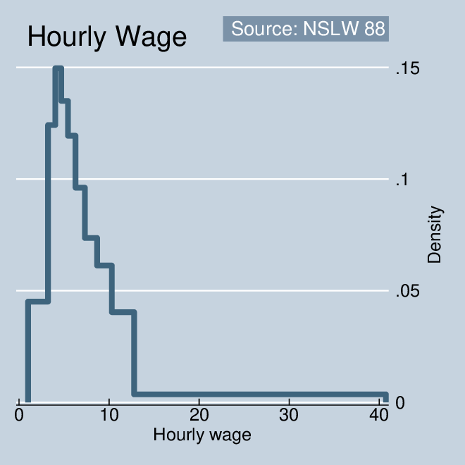
sysuse nlsw88
percentogram wage, bins(10) scheme(economist) title("Hourly Wage") note("Source: NSLW 88")

One final note: this program uses Stata’s frame infrastructure, introduced in version 16 to make it possible to have more than one dataframe in memory. Previously, if we had to create temporary variables they would have had to take their place in the existing dataframe, or we would have had to temporarily save the existing dataframe to disc (using preserve and restore). It’s rather more convenient to do the program’s work in a separate temporary frame, which disappears after use. Here, we create a frame with a temporary name, and then do the key work in the frame `fr' {} block. We begin by creating the necessary number of observations (set obs `nb') in an otherwise empty dataframe, and then process the centile returned results as described above. When the program terminates, the dataframe disappears.

So we have now a working example of creating a new Stata command as an ado-file, and have seen a little of the power of the syntax command (and how it allows the end-user to access the functionality of the underlying commands without the programmer, me, having to code it explicitly). Also, while local macros will probably feel quite odd to users of real programming languages, we see some of their power, not least in accessing results returned by other commands.

For more, go to the Stata documentation, in particular the “Programming Stata” chapter. And note that I’ve said nothing at all about Mata, the matrix language Stata’s internals are written in.

To install this code in Stata do:

net from http://teaching.sociology.ul.ie/statacode
net install percentogram

Postscript

After writing this post, I did a little googling, and came across this “Stata Tip” written by Ben Jann in 2015, discussing a number of similar ideas. Ben mentions in passing that the inimitable Nick Cox wrote a command to do this in 1999, eqprhistogram, which can be installed from SSC:

ssc install eqprhistogram

Thanks to Stas Kolenikov @statstas for helpful comments.